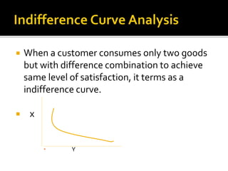
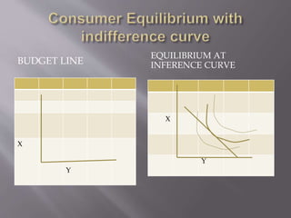
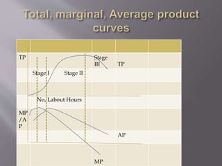
This document provides an overview of concepts related to consumer behavior and production including: - Marginal utility analysis, consumer equilibrium, and indifference curve analysis which are used to understand how consumers maximize utility given budget constraints. - Assumptions of utility analysis including that consumers attempt to maximize well-being, income constraints consumption, and marginal utility diminishes with increasing consumption. - The law of diminishing marginal utility which states that as consumption increases, marginal utility declines. - Consumer equilibrium is reached when marginal utility per rupee is equal across goods. - Indifference curves, their properties including being negatively sloped and convex, and their use in analyzing consumer choice. - Short-run production

1. W. A. Upananda
Former Assistant Professor
11th August, 2019

2.  This session is consisted of:
 Marginal utility analysis
 Consumer equilibrium with Marginal utility
 Indifference curve analysis
 Consumer equilibrium with Indifference curve
analysis

3.  Assumptions in utility analysis
 Consumers attempt to maximize their well-being
which is termed utility (satisfaction)
 Constraints or limitation is the income which
limits consumption
 Any product has substitutes
 Utility is measurable
 Marginal utility of money is constant and marginal
utility is consistent.

4.  Satisfaction you get from several units of the
same commodity could be added up which
makes the total utility.The satisfaction or
utility gained from the last unit is termed
marginal utility.When marginal utility
become zero, the next unit gives negative
satisfaction.
 Mathematically marginal Utility is given as
follows:
 MU= change inTU/Change in Quantity

5. The law of diminishing
marginal utility
Total Utility ‘The law of diminishing
marginal states that as a
person consumes more
and more of a given
commodity of the
commodity eventually
tend to decline’.
Quantity
Marginal
Utility

6.  Consumer reach equilibrium when he spends
his income in such a way that the utility of the
last rupee spent on two commodities is the
same.
 Marginal utility of money expenditure = Marginal
utility of the good/ price of the good.
 Symbolically it could be written as
 Then the money income is

PxMUxMUp /
QyPyQxPx 

7.  When a customer consumes only two goods
but with difference combination to achieve
same level of satisfaction, it terms as a
indifference curve.
 x
 Y

8.  1. Negatively sloped
 2. Convex to the origin
 3. Indifference curves
cannot be intersected.
 4. Downward sloped or left
to right
 5. Amount of one
commodity could be
substitute for another
amount of other
commodity.This is termed
marginal rate of
substitution (MRS).
 Marginal rate of
substitution could be
traced. MRS curve is
downwardly sloped.
 MRS = ∆X/ ∆Y
 X
 Y

9. BUDGET LINE
EQUILIBRIUM AT
INFERENCE CURVE
X
Y
X
Y

10. DEFINING PRODUCTION
 The process of
transformation of inputs
into output.
 For production, one need
fixed inputs such as
buildings and machinery
and variable inputs such as
raw material.
 Fixed inputs do not vary
with the quantity produced
SHORT-RUNANALYSIS
 Q =f (L, K)
 Total production is the total
of goods produced within the
given period of time.
 Average production is the
average production for one
unit of input.
 Marginal product;
 Defined as the change of in
output by the last variable
unit of input added.

11. TP Stage
III TP
Stage I Stage II
No, Labout Hours
MP
/A
P
AP
MP

12.  This section covers 1. cost of production 2. Short-run
cost analysis and Long-run cost analysis.
 Two types of cost Explicit cost (direct cost) and
indirect or Implicit cost.The money spent to buy
machinery is a direct cost while your time is a implicit
cost.
 Fixed cost and variable cost:The cost which does not
change with the output is termed Fixed cost while
cost vary with the output is termed variable cost. Cost
of machinery is fixed cost while cost of input used for
production is a variable cost.

13.  Short-run total cost
(TC)
 TC = TFC+ TVC
 Average cost = TVC/Q
 Marginal cost =
 ∆
TC/∆Q
TC
Cost
TVC
AVC
MC TFC
ATC
QTY

14. Thank you for watching
▪Please do not forget to
comment