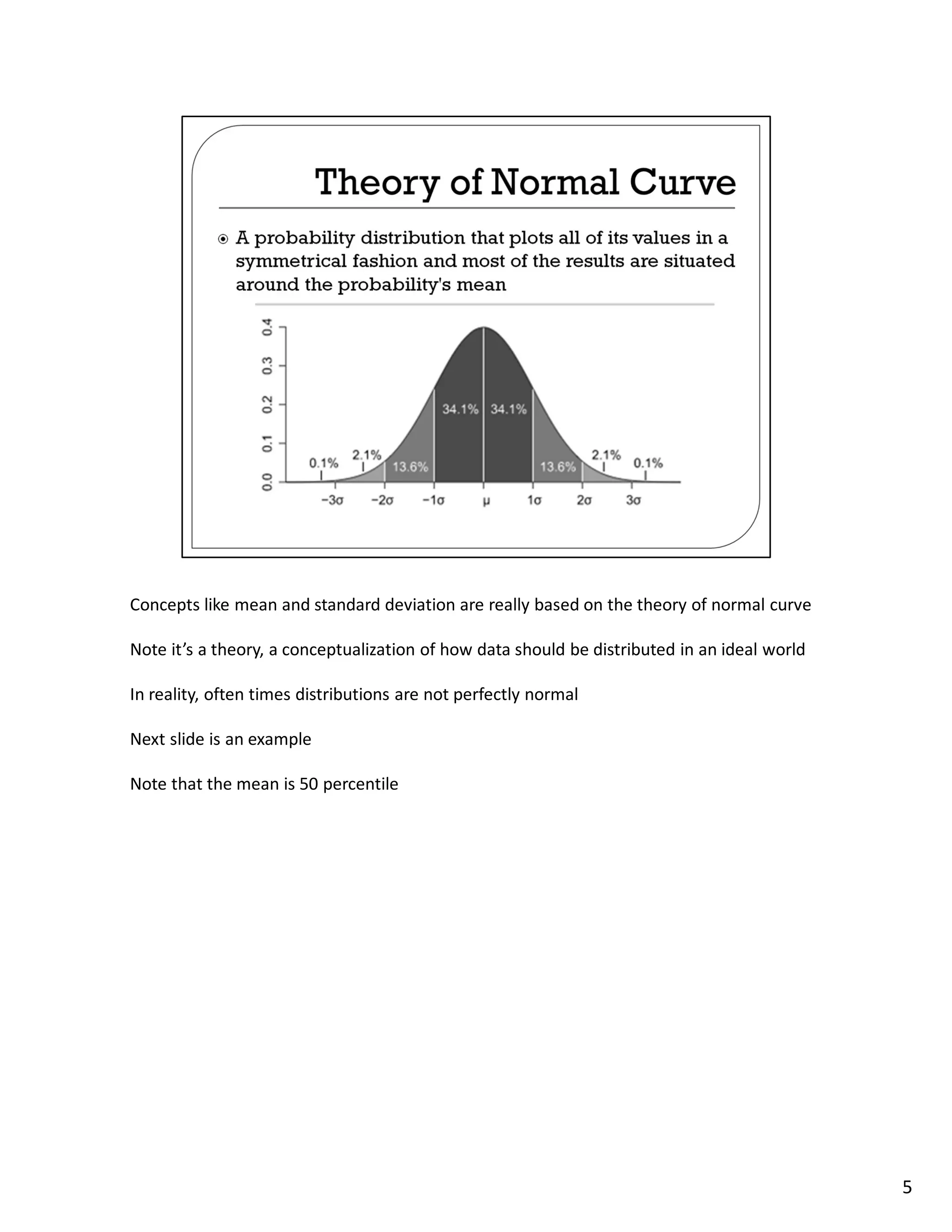
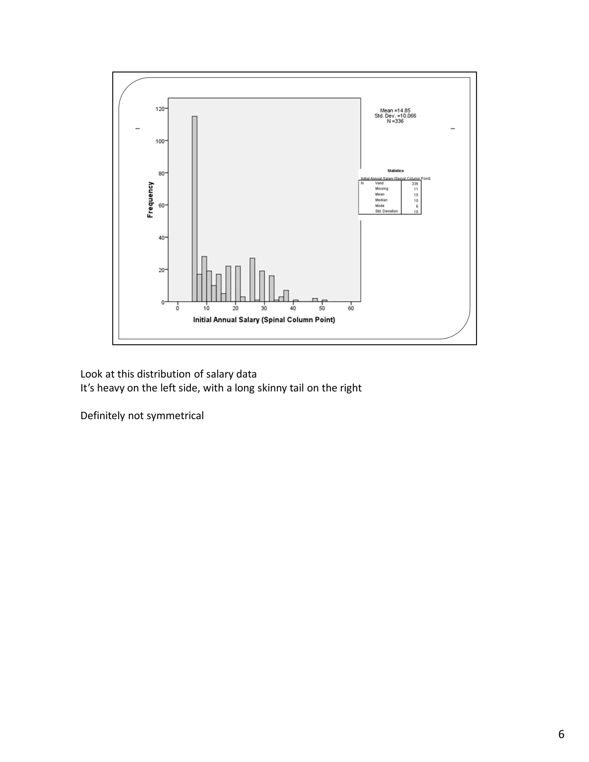
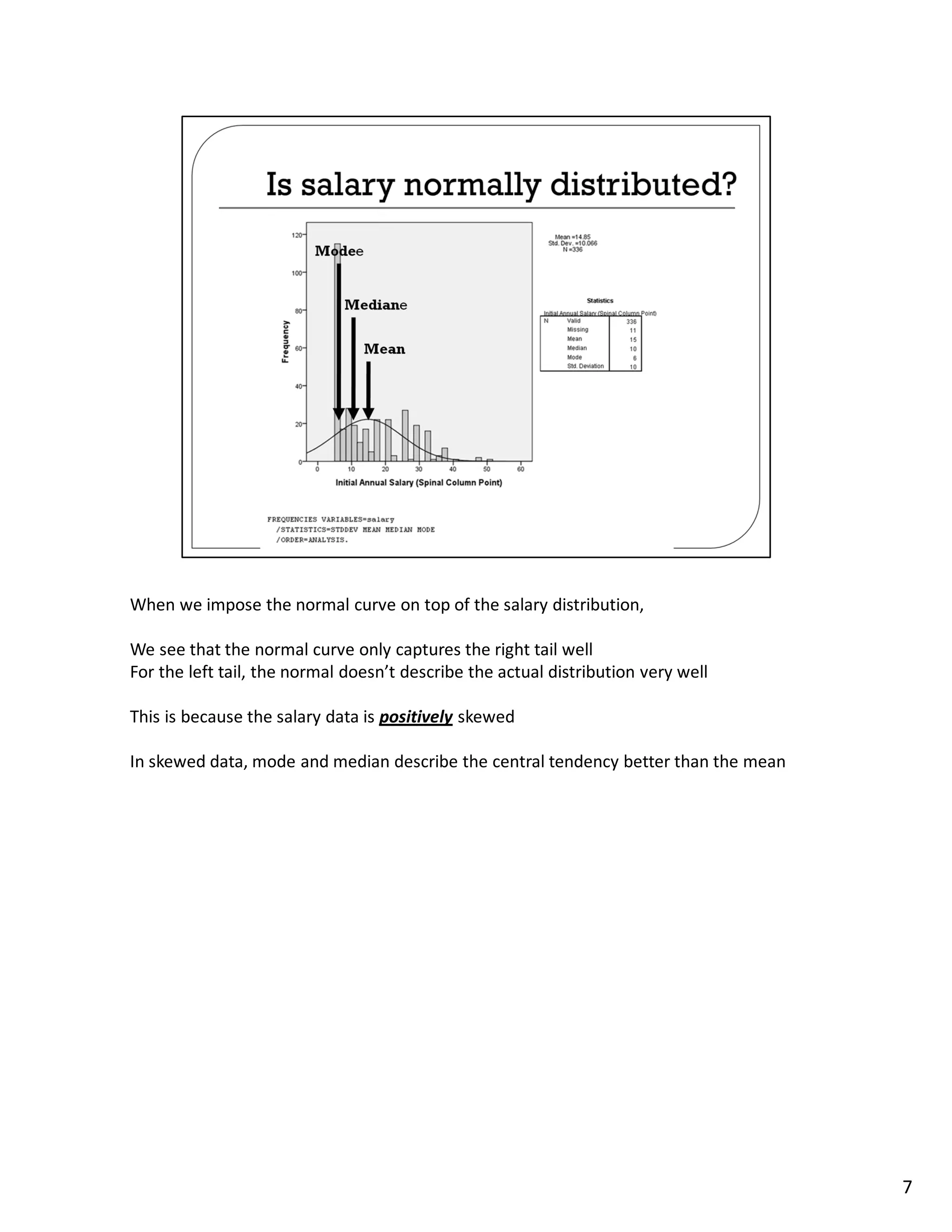
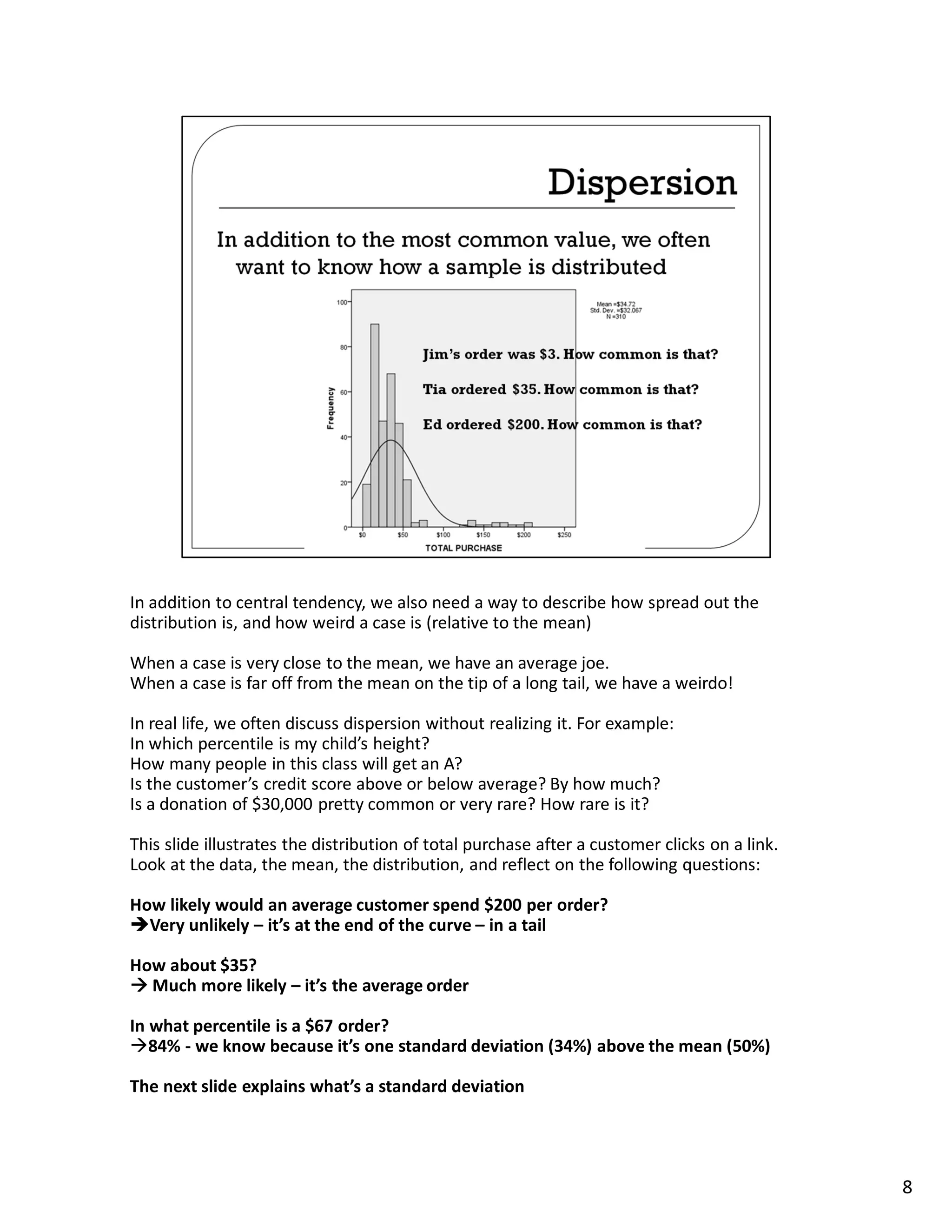
This lecture discusses methods for measuring central tendency and dispersion in statistical samples. Central tendency refers to the most typical or common value in a sample, such as the average or median. Measures of central tendency include the mean, median, and mode. Dispersion describes how spread out or varied the values in a sample are and is measured by the standard deviation. The lecture explains these concepts and provides examples to illustrate how measures of central tendency and dispersion can be used to analyze and understand sample data distributions.

1. This lecture presentation complements Khan’s tutorials
1

2. In this lecture we will discuss the different methods to measure central tendency and
dispersion in a statistical sample.
2

3. Central tendency is just a technical way of saying, what’s typical of this sample? For
example, out of all Carlow students, which gender is the more typical one? Male or female?
Out of all the products listed on Amazon, which is the best seller? And out of all the eBay
listings of “Tickle Me Elmo,” which price is the most common one?
3

4. These three different measures are discussed in detail by Khan Academy. Here are some
brief summaries
We will discuss normal distribution.
One key idea is this:
If the sample is normally distributed, meaning it looks like a symmetrical bell curve, then
mean, median and mode will be the same number.
However, if the sample is skewed either to the left or to the right, then these three
numbers would take on different values.
4

5. Concepts like mean and standard deviation are really based on the theory of normal curve
Note it’s a theory, a conceptualization of how data should be distributed in an ideal world
In reality, often times distributions are not perfectly normal
Next slide is an example
Note that the mean is 50 percentile
5

6. Look at this distribution of salary data
It’s heavy on the left side, with a long skinny tail on the right
Definitely not symmetrical
6

7. When we impose the normal curve on top of the salary distribution,
We see that the normal curve only captures the right tail well
For the left tail, the normal doesn’t describe the actual distribution very well
This is because the salary data is positively skewed
In skewed data, mode and median describe the central tendency better than the mean
7

8. In addition to central tendency, we also need a way to describe how spread out the
distribution is, and how weird a case is (relative to the mean)
When a case is very close to the mean, we have an average joe.
When a case is far off from the mean on the tip of a long tail, we have a weirdo!
In real life, we often discuss dispersion without realizing it. For example:
In which percentile is my child’s height?
How many people in this class will get an A?
Is the customer’s credit score above or below average? By how much?
Is a donation of $30,000 pretty common or very rare? How rare is it?
This slide illustrates the distribution of total purchase after a customer clicks on a link.
Look at the data, the mean, the distribution, and reflect on the following questions:
How likely would an average customer spend $200 per order?
Very unlikely – it’s at the end of the curve – in a tail
How about $35?
Much more likely – it’s the average order
In what percentile is a $67 order?
84% - we know because it’s one standard deviation (34%) above the mean (50%)
The next slide explains what’s a standard deviation
8

9. Standard deviation is a standardized measure of dispersion
It tells you whether the distribution is short and fat (with a big standard distribution) or tall
and skinny (with a small standard distribution)
The calculation is explained well by Khan
The basic idea to take away is:
The standard deviation tells you, on average, how far away the data points are from the
mean
For example, let’s say that the Steelers have an average score of 25 per game, and the
standard deviation is 1. Let’s also say that the Greenbay Packers have an average score of
25 per game, and a standard deviation of 7.
In this example, both teams are comparable in terms of average scores, but the Steelers
have a much smaller standard deviation. This means the Steelers’ performance is pretty
consistent over time, their scores may be above or below 25, but only by 1-2 points on
average. If you plot their scores on a chart, you would see that most of them pack around
25, with a nice narrow distribution that peaks around 25.
In contrast, the Packers may average around 25, but their performance varies widely from
game to game. One day they may score 18 (25-7) and the next day they may score 32
(25+7) If you plot their widely varied scores on a chart, you would get a short and fat
9

10. distribution.
(Go Steelers Go!)
9

11. What are practical ways to use the standard deviation?
With a normal distribution, the mean divides it up evenly in the middle. The portion below
the mean covers 50% of the population, whereas the portion above the mean also covers
50% of the population.
The first standard deviation away from the mean covers 34% of the distribution.
In other words, 1 standard deviation above the mean is 50% + 34% which is 84 percentile
Let’s say that the average weight for a one year old is 25 pounds, and a standard deviation
of 2 pounds.
Connor is 23 pounds. That’s 1 standard deviation below the mean. In other words he is
50%-34% or 16th percentile of the population
Nardia is 27 pounds. That’s 1 standard deviation above the mean. In other words she is
50%+34% or 84th percentile of the population
The entire distribution is covered by roughly 6 standard deviations – 3 above the mean and
3 below the mean
Hence the name of the quality management program “Six Sigma”
10

12. More examples:
Given a mean and a standard deviation score, you have a pretty good idea of what the
distribution is like – is it fat and short, or tall and skinny?
We can then map out individual scores on the distribution and tell the average joes from
the weirdos!
11

13. The Z score is the number of standard deviations fro the mean
With our previous example, Connor would have a Z score of 1, while Nardia has a Z score of
negative 1.
The average joes would have close to zero z scores (e.g., 0.0006, -.0029)
Whereas the weirdos have extremely large or small z scores (e.g., 3.07, -2.99)
Again -
The z score is the number of standard deviations a data point is away from the mean
Let's say that the average weight for all American women is 150, and the standard
deviation is 20.
If your weight is 130, then your z score is -1, because you're exactly 1 standard deviation
below the mean.
If Peggy's weight is 170, then her z score is 1, because she is exactly 1 standard deviation
above the mean.
12

14. Questions? Schedule a chat/phone meeting with the instructor for more assistance
13