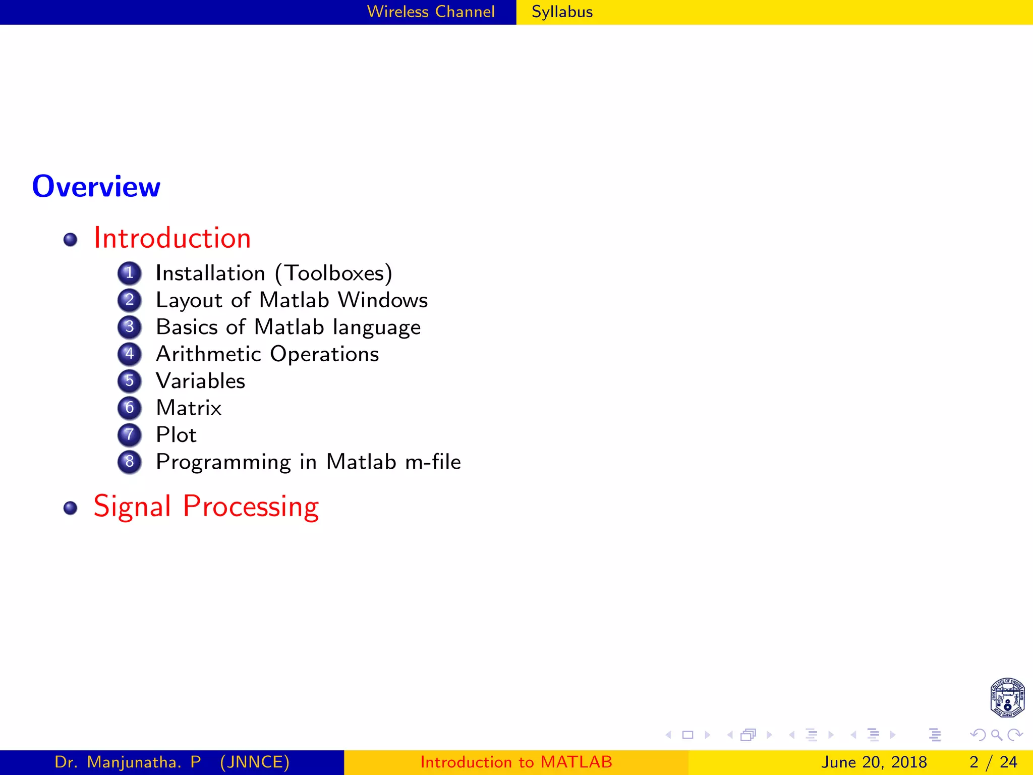
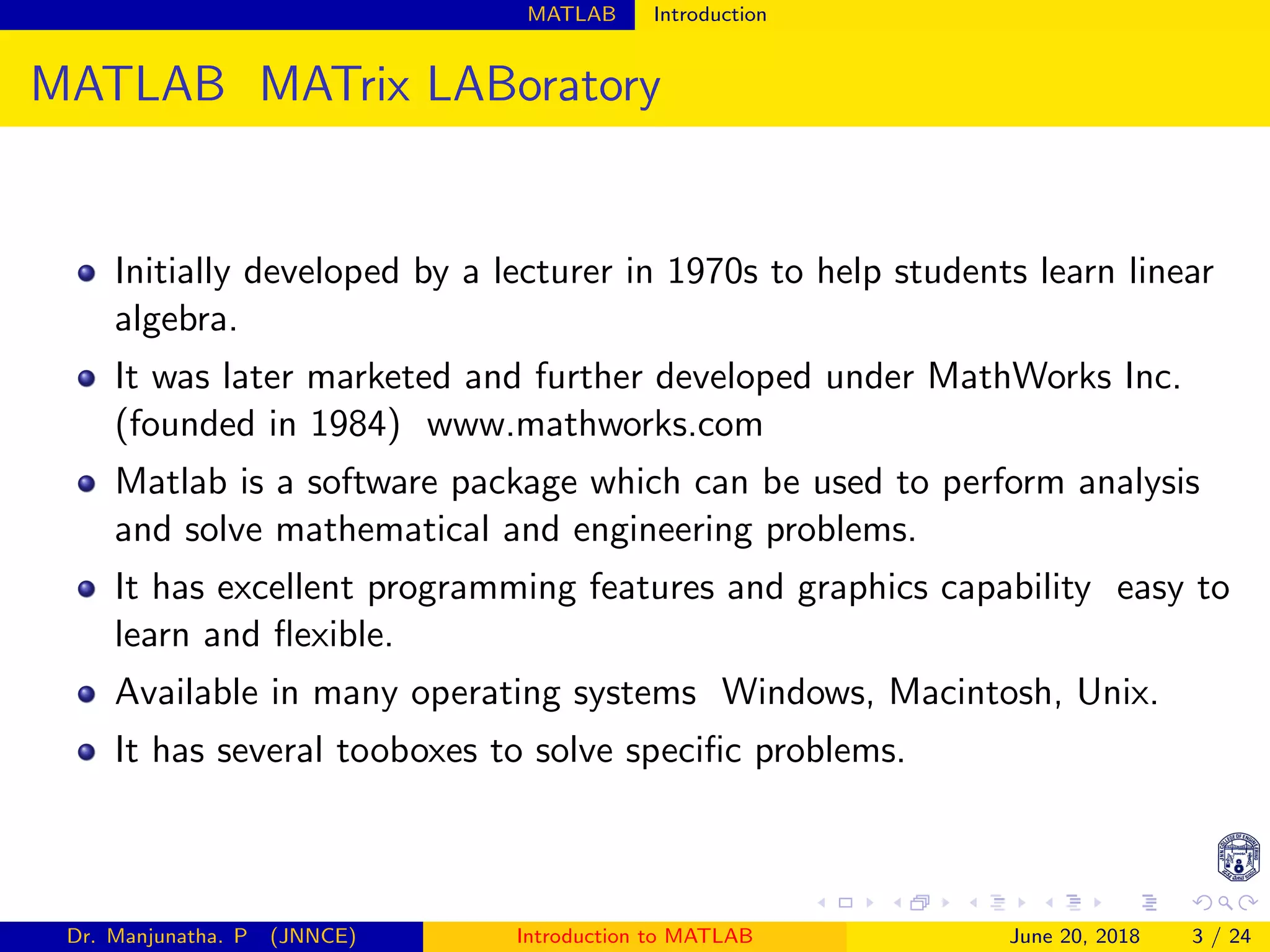
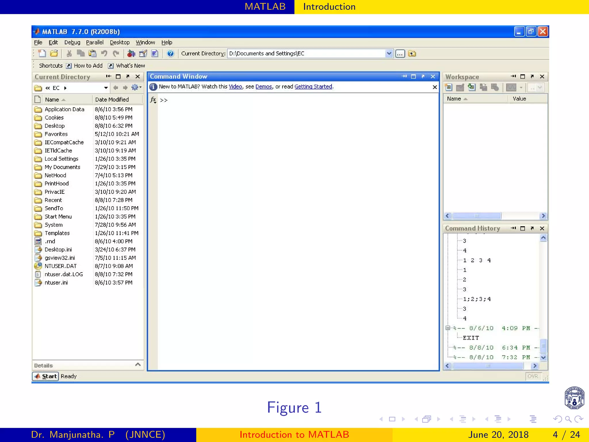
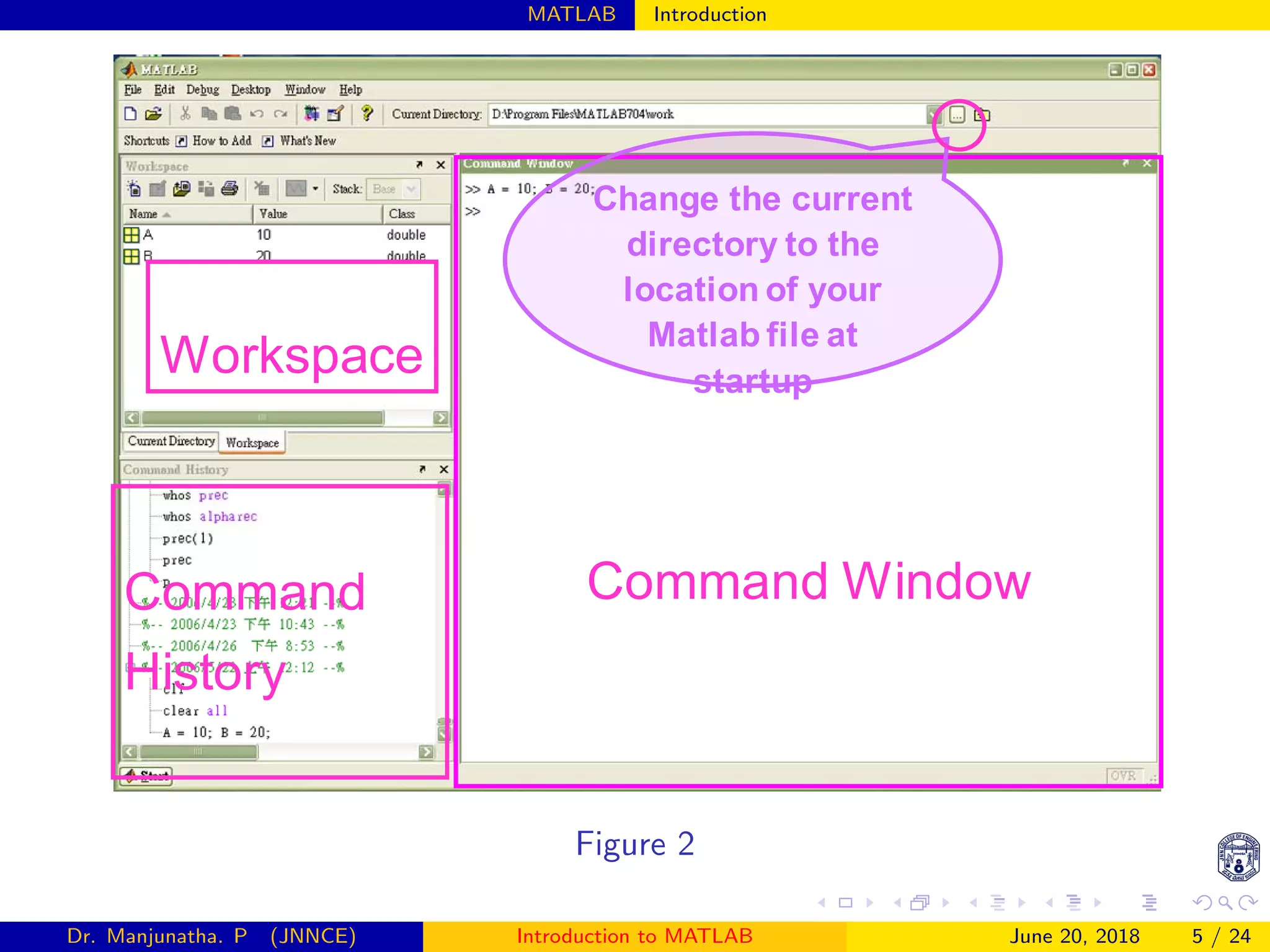
The document provides an introduction and overview of MATLAB. It discusses that MATLAB was initially developed as a tool to help students learn linear algebra and is now a widely used software package for engineering and mathematical problems. The document then covers various MATLAB windows and basics like variables, matrices, plot commands, m-files, and flow control structures like for loops and if/else statements. It also provides examples of plotting functions and creating graphs with labels and titles.

1. Introduction to MATLAB
Dr. Manjunatha. P
manjup.jnnce@gmail.com
Professor
Dept. of ECE
J.N.N. College of Engineering, Shimoga
June 20, 2018

2. Wireless Channel Syllabus
Overview
Introduction
1 Installation (Toolboxes)
2 Layout of Matlab Windows
3 Basics of Matlab language
4 Arithmetic Operations
5 Variables
6 Matrix
7 Plot
8 Programming in Matlab m-file
Signal Processing
Dr. Manjunatha. P (JNNCE) Introduction to MATLAB June 20, 2018 2 / 24

3. MATLAB Introduction
MATLAB MATrix LABoratory
Initially developed by a lecturer in 1970s to help students learn linear
algebra.
It was later marketed and further developed under MathWorks Inc.
(founded in 1984) www.mathworks.com
Matlab is a software package which can be used to perform analysis
and solve mathematical and engineering problems.
It has excellent programming features and graphics capability easy to
learn and flexible.
Available in many operating systems Windows, Macintosh, Unix.
It has several tooboxes to solve specific problems.
Dr. Manjunatha. P (JNNCE) Introduction to MATLAB June 20, 2018 3 / 24

4. MATLAB Introduction
Figure 1
Dr. Manjunatha. P (JNNCE) Introduction to MATLAB June 20, 2018 4 / 24

5. MATLAB Introduction
Command Window
Workspace
Command
History
Change the current
directory to the
location of your
Matlab file at
startup
Figure 2
Dr. Manjunatha. P (JNNCE) Introduction to MATLAB June 20, 2018 5 / 24

6. MATLAB Introduction
Command Window
Workspace
1 view program variables
2 clear to clear
3 double click on a variable to see it in the Array Editor
Command History
1 view past commands
2 save a whole session using diary
Launch Pad
1 access tools,
2 demos and documentation
Dr. Manjunatha. P (JNNCE) Introduction to MATLAB June 20, 2018 6 / 24

7. MATLAB Introduction
Matlab prompts >> when it is ready to accept a command.
To end a matlab session type quit or exit at the matlab prompt.
Type help at the matlab prompt, to get help topics.
Variables
1 Variables in matlab are named objects that are assigned using the equals sign =.
2 They are limited to 31 characters and can contain upper and lowercase letters, any
number of characters, and numerals.
3 They may not start with a numeral.
4 matlab is case sensitive: A and a are different variables.
5 who lists in alphabetical order all variables in the currently active workspace.
6 clear removes all variables from the workspace. This frees up system memory.
Dr. Manjunatha. P (JNNCE) Introduction to MATLAB June 20, 2018 7 / 24

8. MATLAB Useful Commands
Some Useful Commands
clc clear command window
clear all clear all variables in the memory
close all closes all the opened windows
quit, exit quit MATLAB
who what variables in memory
whos all size of the variables
; suppress printing
% comments (matlab will not read)
sin(C) sine of each entry of matrix C
exp(C) exponential of each entry of C
real(C) real part of each entry of C
ceil(C) round each Cs entry up
floor(C) round each Cs entry down
sqrt(C) square root of each entry of C
Request user input
x=input(’Enter x: ’)
Dr. Manjunatha. P (JNNCE) Introduction to MATLAB June 20, 2018 8 / 24

9. MATLAB Working with m file
Working with Script M-file description
To work with Script M-file
File ⇒ New blank m file
In the opened window write the script file
save the m file with suitable file name
While saving or creating new m file: It should not start with numerals, don’t use any build
in command or function name like conv, disp corr,
Dr. Manjunatha. P (JNNCE) Introduction to MATLAB June 20, 2018 9 / 24

10. MATLAB Operators
Arithmetic Operators
+ Addition
− Subtraction
∗ Multiplication
/ Division
∧ Power
Complex conjugate transpose
y = 2 + 3
y = 2 − 3
y = 2 ∗ 3
y = 4/2
y = 2 ∧ 3
x = [1, 2, 3], y = x
Relational and logical Operators
== Equal
∼= Not equal
< Less than
<=Less than or equal
> Greater than
>=Greater than or equal
& AND
! OR
∼ NOT
clc; clear all; close all;
a=5; b=33; c=65;
if a==b
y=30
else y=65
end
if a~=b & b~=30
y=100
else y=500
end
Dr. Manjunatha. P (JNNCE) Introduction to MATLAB June 20, 2018 10 / 24

11. MATLAB Vectors and Matrices
Vectors and Matrices
Row vector: A row vector: values
are separated by spaces or comma
A = [1 2 3 4 5]
Column vector: A column vector:
values are separated by semicolon
(;)
B = [1;2;4;6;8]





1
2
4
6
8





Matrices


1 2 3
4 5 6
7 8 9


A=[1 2 3;4 5 6;7 8 9]
Each row is separated by space or comma
and next row elements are created by plac-
ing semicolon(;)
Special matrices
zeros(1,3)
0 0 0
zeros(3,3)


0 0 0
0 0 0
0 0 0


ones(3,3)


1 1 1
1 1 1
1 1 1


Finding the length of the vector
A=[1 2 3 4 5 6 7 8 9]
N=length(A)
=9
Display text or array
disp(A)
disp(’Length of the sequence is ’)
Dr. Manjunatha. P (JNNCE) Introduction to MATLAB June 20, 2018 11 / 24

12. MATLAB Vectors and Matrices
To access elements in a matrix or a vector
A = [2 4 5 7 8]
To access the second element in an
array use A(2)
=4
Consider a matrix
A = [1 2 3; 4 5 6; 7 8 9]
A =


1 2 3
4 5 6
7 8 9


To access the first row elements in a
matrix A(1,:) is
[1 2 3]
To access the second column elements
in a matrix
A(:,2) is
2
3
8
Performing operations to every
element of a matrix
A+3 

3 5 6
7 8 9
10 11 12


A-3 

−1 0 1
2 3 4
5 6 7


Multiplying every element of a matrix
by 2
A ∗ 2 

2 4 6
8 10 12
14 16 18


Flip matrix left to right
A = [2 4 5 7 8]
B = fliplr(A)
Dr. Manjunatha. P (JNNCE) Introduction to MATLAB June 20, 2018 12 / 24

13. MATLAB Vectors and Matrices
Difference between squaring matrix and squaring elements in each matrix
A = [1 2 3; 4 5 6; 7 8 9]
A =


1 2 3
4 5 6
7 8 9


To square every element in
matrix, use the elementwise
operator .∧
B = A. ∧ 2
B = A.∧2 =


1 4 9
16 25 36
49 64 81


B = A ∧ 2 = A ∗ A =
B = A∧2


30 36 42
66 81 96
102 126 150


Performing operations to every element of a matrix
B = [1 1 1; 2 2 2; 3 3 3]
A =


1 2 3
4 5 6
7 8 9

 B =


1 1 1
2 2 2
3 3 3


C=A*B


1 2 3
4 5 6
7 8 9




1 1 1
2 2 2
3 3 3

 =


14 14 14
32 32 32
50 50 50


C=A.*B


1x1 2x1 3x1
4x2 5x2 6x2
7x3 8x3 9x3

 =


1 2 3
8 10 12
21 24 27


Dr. Manjunatha. P (JNNCE) Introduction to MATLAB June 20, 2018 13 / 24

14. MATLAB Flow Control Constructs
Flow Control Constructs
for, while, if
Fixed repetition: the for loop
Multiple options: the if/elseif/else
Indefinite repetition: the while loop
Single decision: the if/else construct
for loop
for i = 1:m
loop body statements
each statement executed m times
end
for i = k:l:m
from k to m in steps of l
end
Example:
Calculating sum from 1 to 10
clc; clear all; close all;
sum=0;
for i=1:10
sum=sum+i
end
Nesting for-loop
clc; clear all; close all;
m=3;
A = zeros(m,m)
for i = 1:m
for j = 1:m
A(i,j) = 2
end
end
Dr. Manjunatha. P (JNNCE) Introduction to MATLAB June 20, 2018 14 / 24

15. MATLAB Flow Control Constructs
while construct:
while < condition >
every statement will be executed until con-
dition is not satisfied
end
clc; clear all; close all;
% sum of 1 to 10
a = (1:10);
s = 0;
j=1; % set the test variable
while j < 11 % check the condition
s = s+a(j)
j = j+1; % update test variable
end
clc; clear all; close all;
% sum of a 1 to 10
a = (1:10);
s = 0;
j=1; % set the test variable
for j=1:10
s = s+a(j)
end
Example:
Calculating sum from 1 to 10
clc; clear all; close all;
sum=0;
for i=1:10
sum=sum+i
end
Nesting for-loop
clc; clear all; close all;
m=3;
A = zeros(m,m)
for i = 1:m
for j = 1:m
A(i,j) = 2
end
end
Dr. Manjunatha. P (JNNCE) Introduction to MATLAB June 20, 2018 15 / 24

16. MATLAB Flow Control Constructs
clc; clear all; close all;
marks=[95 55 65 85 35 25];
m=length(marks);
for j=1:m
if marks(j)>=90
grade(j)=’A’;
elseif marks(j)>=80
grade(j)=’B’;
elseif marks(j)>=70
grade(j)=’C’;
elseif marks(j)>=60
grade(j)=’D’;
elseif marks(j)>=50
grade(j)=’E’ ;
elseif marks(j)<=40
grade(j)=’F’
end
end
Dr. Manjunatha. P (JNNCE) Introduction to MATLAB June 20, 2018 16 / 24

17. MATLAB Graph Functions (summary)
Graphics - 2D Plots
Command Description
plot linear plot
stem Plot discrete sequence data
grid add grid lines
xlabel add X axis label
ylabel add Y axis label
figure create new figure
title add graph title
subplot divide figure
pause wait for user response
0 1 2 3 4 5 6 7
−1
−0.8
−0.6
−0.4
−0.2
0
0.2
0.4
0.6
0.8
1
clc; clear all; close all;
x = 0:pi/1000:2*pi;
y = sin(x);
plot(x,y)
xlabel(’x = 0:2pi’)
ylabel(’Sine of x’)
title(’Plot of the Sine Function’)
figure
x1 = 0:pi/30:2*pi;
y1 = sin(x1);
stem(x1,y1)
0 1 2 3 4 5 6 7
−1
−0.8
−0.6
−0.4
−0.2
0
0.2
0.4
0.6
0.8
1
x = 0:2π
Sineofx
Plot of the Sine Function
Dr. Manjunatha. P (JNNCE) Introduction to MATLAB June 20, 2018 17 / 24

18. MATLAB Graph Functions (summary)
clc; clear all; close all;
x = 0:pi/1000:2*pi;
y = sin(x);
plot(x,y)
xlabel(’x = 0:2pi’)
ylabel(’Sine of x’)
title(’Plot of the Sine Function’)
figure
x1 = 0:pi/30:2*pi;
y1 = sin(x1);
stem(x1,y1)
figure
subplot(2,1,1)
plot(x,y)
subplot(2,1,2)
stem(x1,y1)
figure
subplot(1,2,1)
plot(x,y)
subplot(1,2,2)
stem(x1,y1)
0 1 2 3 4 5 6 7
−1
−0.5
0
0.5
1
0 1 2 3 4 5 6 7
−1
−0.5
0
0.5
1
Figure 3: Subplot demo
0 2 4 6 8
−1
−0.8
−0.6
−0.4
−0.2
0
0.2
0.4
0.6
0.8
1
0 2 4 6 8
−1
−0.8
−0.6
−0.4
−0.2
0
0.2
0.4
0.6
0.8
1
Figure 4: Subplot demo
Dr. Manjunatha. P (JNNCE) Introduction to MATLAB June 20, 2018 18 / 24

19. MATLAB Graph Functions (summary)
Graphics - 2D Plots
clc; clear all; close all;
t = 0:0.001:1;
y1=sin(2*pi*50*t);
y2 = 2*sin(2*pi*120*t);
y = sin(2*pi*50*t) + 2*sin(2*pi*120*t);
subplot(3,1,1)
plot(t(1:50),y1(1:50));
subplot(3,1,2)
plot(t(1:50),y2(1:50));
subplot(3,1,3)
plot(t(1:50),y(1:50));
0 0.005 0.01 0.015 0.02 0.025 0.03 0.035 0.04 0.045 0.05
−1
0
1
0 0.005 0.01 0.015 0.02 0.025 0.03 0.035 0.04 0.045 0.05
−2
0
2
0 0.005 0.01 0.015 0.02 0.025 0.03 0.035 0.04 0.045 0.05
−5
0
5
clc; clear all; close all;
fs = 100;
t = 0:1/fs:1;
x = sin(2*pi*t*3)+.25*sin(2*pi*t*40);
b = ones(1,10)/10; % 10 point averaging
y = filter(b,1,x);
plot(t,x,’b’,t,y,’r’,’linewidth’,2)
legend(’noisy signal’,’filtered signal’
0 0.1 0.2 0.3 0.4 0.5 0.6 0.7 0.8 0.9 1
−1.5
−1
−0.5
0
0.5
1
1.5
noisy signal
filtered signal
Dr. Manjunatha. P (JNNCE) Introduction to MATLAB June 20, 2018 19 / 24

20. MATLAB Graph Functions (summary)
Colors, Markers and Line Types
symbol Color symbol Marker symbol Line
y yellow • Point - solid
m magenta ◦ circle : dotted
c cyan × x mark −. dot dash
r red + plus − − dashed
g green star
b blue s square
k black d diamond
v triangle down
clc; clear all; close all;
x=[0:0.1:2*pi];
subplot(2,1,1)
plot(x,sin(x),’linewidth’,2)
subplot(2,1,2)
plot(x,sin(x),’.’,x,cos(x),’o’,’linewidth’,2)
0 1 2 3 4 5 6 7
−1
−0.5
0
0.5
1
0 1 2 3 4 5 6 7
−1
−0.5
0
0.5
1
Dr. Manjunatha. P (JNNCE) Introduction to MATLAB June 20, 2018 20 / 24

21. MATLAB Graph Functions (summary)
clc; clear all; close all;
clc; clear all; close all;
x=[0:0.1:2*pi];
y=sin(x);
z=cos(x);
d=degtorad(45);
p=sin(x+d);
subplot(3,1,1)
plot(x,y,’linewidth’,2)
subplot(3,1,2)
plot(x,z,’r’,’linewidth’,2)
subplot(3,1,3)
plot(x,p,’m:o’)
title(’Sample Plot’,’fontsize’,14);
xlabel(’X values’,’fontsize’,14);
ylabel(’P values’,’fontsize’,14);
% legend(’Y data’,’Z data’,’p data’)
grid on
0 1 2 3 4 5 6 7
−1
0
1
0 1 2 3 4 5 6 7
−1
0
1
0 1 2 3 4 5 6 7
−1
0
1
Sample Plot
X values
Pvalues
Dr. Manjunatha. P (JNNCE) Introduction to MATLAB June 20, 2018 21 / 24

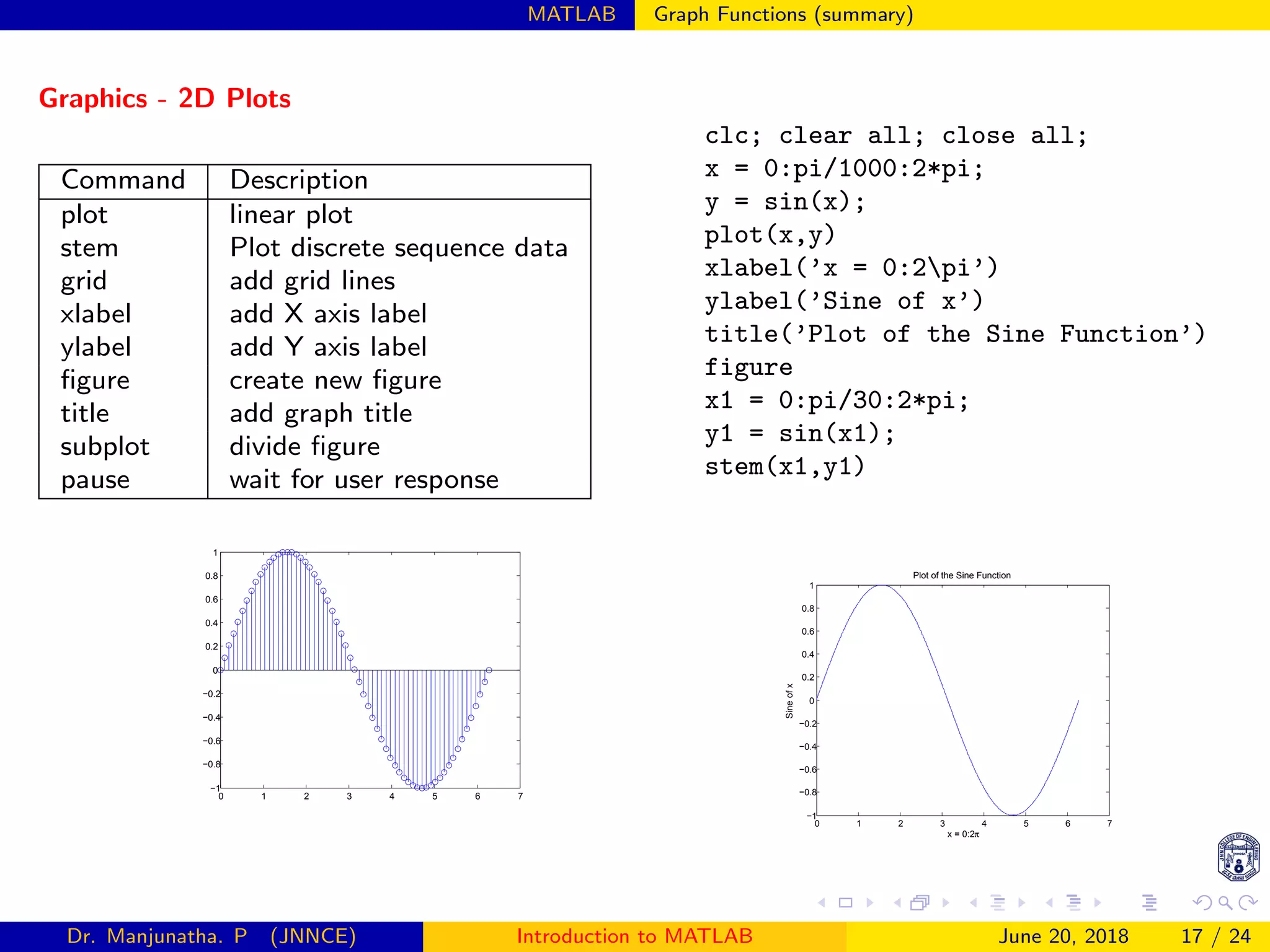
22. MATLAB Graph Functions (summary)
Colors, Markers and Line Types
Command Description
plot linear plot
stem discrete plot
grid add grid lines
xlabel add X axis label
ylabel add Y axis label
figure create new figure
title add graph title
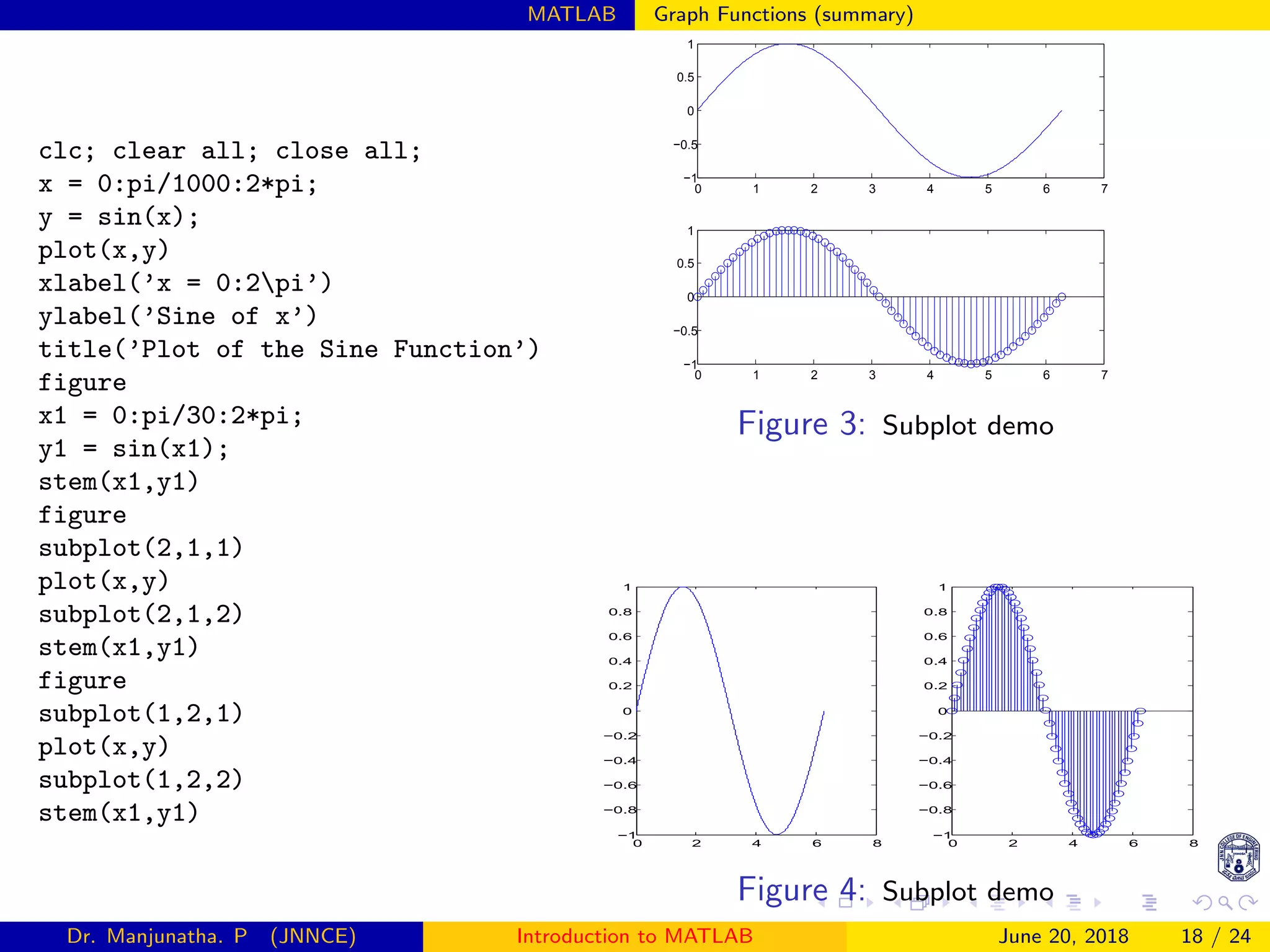
subplot divide figure
pause wait for user response
clc; clear all; close all;
x=[0:0.01:2*pi];
y=sin(x);
z=cos(x);
d=degtorad(45);
p=sin(x+d);
plot(x,y,x,z,x,p,’linewidth’,2)
title(’Sample Plot’,’fontsize’,14);
xlabel(’X values’,’fontsize’,14);
ylabel(’Y values’,’fontsize’,14);
legend(’Y data’,’Z data’,’p data’)
grid on
0 1 2 3 4 5 6 7
−1
−0.8
−0.6
−0.4
−0.2
0
0.2
0.4
0.6
0.8
1
Sample Plot
X values
Yvalues
Y data
Z data
P data
Dr. Manjunatha. P (JNNCE) Introduction to MATLAB June 20, 2018 22 / 24

23. MATLAB Graph Functions (summary)
Find the frequency components of a signal buried in noise. Consider data sampled at 1000
Hz. Form a signal consisting of 50 Hz and 120 Hz sinusoids and corrupt the signal with
random noise.
clc; clear all; close all;
t = 0:0.001:0.6;
x = sin(2*pi*50*t) + sin(2*pi*120*t); %signal
y = x + 2*randn(1,length(t));%adding noise
Y = fft(y,512); %discrete Fourier transform
Pyy = Y.*conj(Y) / 512;% power spectral density
f = 1000*(0:255)/512;
figure
subplot(2,1,1)
plot(y(1:50));
title(’signal +noise’,’fontsize’,14);
subplot(2,1,2)
plot(f,Pyy(1:256))
title(’FFT of the signal’,’fontsize’,14);
0 5 10 15 20 25 30 35 40 45 50
−5
0
5
10
signal +noise
0 50 100 150 200 250 300 350 400 450 500
0
20
40
60
80
FFT of the signal
Dr. Manjunatha. P (JNNCE) Introduction to MATLAB June 20, 2018 23 / 24

24. MATLAB Graph Functions (summary)
3D plot
clc; clear all; close all;
[X,Y] = meshgrid(1:3,10:14)
[X,Y] = meshgrid(-2:.2:2, -2:.2:2);
Z = X .* exp(-X.^2 - Y.^2);
surf(X,Y,Z)
−2
−1
0
1
2
−2
−1
0
1
2
−0.5
0
0.5
Dr. Manjunatha. P (JNNCE) Introduction to MATLAB June 20, 2018 24 / 24