Downloaded 19 times
![A quick guide on how to use Matlab netCDF functions
Prepared by HP Huang (hp.huang@asu.edu), Sept 2009. Revised March 2015. Please email HPH for
any questions/comments.
A netCDF file contains two parts: A "header" that describes the names, dimensions, etc., of the
variables stored in the file, and the main body that contains the real data. To process a netCDF file, we
need to first extract the information in the header and determine what portion/segment of the data we
want to use. This is usually done by using a set of stand-alone tools. This is, in fact, the more tedious
task which we will discuss in Part (A). Once the content of a netCDF file is known, it is rather
straightforward to read the data as will be discussed in Part (B).
(A) Inspect the content of a netCDF file
We will use the netCDF data file, precip.mon.ltm.nc, as an example to explain how the Matlab
functions work. This file, extracted and downloaded from the the NOAA ESRL-PSD web portal
(www.esrl.noaa.gov/psd), contains the CMAP gridded data for the long-term mean of monthly
precipitation for the global domain. It contains the values of precipitation rate on a regular longitude-
latitude grid for the climatological means for January, February, ..., December.
Step 0: Display/check the header of the netCDF file
ncdisp('precip.mon.ltm.nc')
The output is listed in Appendix A.
Remark: The ncdisp command "dumps" out the whole header, which contains the essential information
about the variables and their dimensions in the netCDF file. Running ncdisp is equivalent to running
"ncdump -c" (see Appendix B) on Linux-based platforms. It is strongly recommended that the
information in the header be examined before one uses the data in a netCDF file. In fact, just by
carefully inspecting the header, one can skip many steps discussed in Step 2-4 in this section.
Step 1: Open the file
ncid1 = netcdf.open('precip.mon.ltm.nc','NC_NOWRITE')
Remark: This command "opens" a netCDF file named precip.mon.ltm.nc and assigns a file number to
it. This file number is the sole output of the function and is put into our variable, ncid1, for later uses.
The option 'NC_NOWRITE' designates that the file is read-only (that is what we need for now).
Steps 2-4 are often not necessary if one has already obtained the needed information about
specific variables by running ncdisp in Step 0.
Step 2: Inspect the number of variables and number of dimensions, etc., in the file
[ndim, nvar, natt, unlim] = netcdf.inq(ncid1)
ndim = 3
1](https://image.slidesharecdn.com/matlabnetcdfguide-160117203239/85/Matlab-netcdf-guide-1-320.jpg)
![A quick guide on how to use Matlab netCDF functions
Prepared by HP Huang (hp.huang@asu.edu), Sept 2009. Revised March 2015. Please email HPH for
any questions/comments.
A netCDF file contains two parts: A "header" that describes the names, dimensions, etc., of the
variables stored in the file, and the main body that contains the real data. To process a netCDF file, we
need to first extract the information in the header and determine what portion/segment of the data we
want to use. This is usually done by using a set of stand-alone tools. This is, in fact, the more tedious
task which we will discuss in Part (A). Once the content of a netCDF file is known, it is rather
straightforward to read the data as will be discussed in Part (B).
(A) Inspect the content of a netCDF file
We will use the netCDF data file, precip.mon.ltm.nc, as an example to explain how the Matlab
functions work. This file, extracted and downloaded from the the NOAA ESRL-PSD web portal
(www.esrl.noaa.gov/psd), contains the CMAP gridded data for the long-term mean of monthly
precipitation for the global domain. It contains the values of precipitation rate on a regular longitude-
latitude grid for the climatological means for January, February, ..., December.
Step 0: Display/check the header of the netCDF file
ncdisp('precip.mon.ltm.nc')
The output is listed in Appendix A.
Remark: The ncdisp command "dumps" out the whole header, which contains the essential information
about the variables and their dimensions in the netCDF file. Running ncdisp is equivalent to running
"ncdump -c" (see Appendix B) on Linux-based platforms. It is strongly recommended that the
information in the header be examined before one uses the data in a netCDF file. In fact, just by
carefully inspecting the header, one can skip many steps discussed in Step 2-4 in this section.
Step 1: Open the file
ncid1 = netcdf.open('precip.mon.ltm.nc','NC_NOWRITE')
Remark: This command "opens" a netCDF file named precip.mon.ltm.nc and assigns a file number to
it. This file number is the sole output of the function and is put into our variable, ncid1, for later uses.
The option 'NC_NOWRITE' designates that the file is read-only (that is what we need for now).
Steps 2-4 are often not necessary if one has already obtained the needed information about
specific variables by running ncdisp in Step 0.
Step 2: Inspect the number of variables and number of dimensions, etc., in the file
[ndim, nvar, natt, unlim] = netcdf.inq(ncid1)
ndim = 3
1](https://image.slidesharecdn.com/matlabnetcdfguide-160117203239/75/Matlab-netcdf-guide-1-2048.jpg)
![nvar = 4
natt = 6
unlim = 2
Remark: After opening a file and obtaining its "file number", we next inquire what's in the file. The
output of the function, netcdf.inq, is a four-element array that contains the number of dimension,
number of variable, number of attribute, etc. (Let's focus on the first two elements for now.) From those
outputs, we learned that the file, "precip.mon.ltm.nc", contains 4 variables (nvar = 4) and maximum of
3 dimensions (ndim = 3).
Step 3: Extract further information for each "dimension"
[dimname, dimlength] = netcdf.inqDim(ncid1, 0)
dimname = lon
dimlength = 144
[dimname, dimlength] = netcdf.inqDim(ncid1, 1)
dimname = lat
dimlength = 72
[dimname, dimlength] = netcdf.inqDim(ncid1, 2)
dimname = time
dimlength = 12
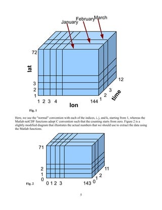
Remark: From Step 2, we learned that there can be maximum of three dimensions for any variable
stored in 'precip.mon.ltm.nc'. We then call the function, netcdf.inqDim(ncid, dimid), to ask about the
detail of each dimension, one at a time. Note that the parameter, dimid, runs from 0 to 2 instead of 1
to 3 (dimension number zero, dimid = 0, corresponds to the 1st dimension; dimension number one,
dimid = 1, corresponds to the 2nd dimension, and so on). This is because Matlab netCDF utilities
adopt the convention of C language, in which the counting of numbers often starts from zero instead of
one. Here, we stop at dimension number 2 (or, the 3rd dimension) because from Step 2 we already
determined that the maximum number of dimension is 3. From this step, we know that the coordinate
for the first dimension is stored in an array called "lon" with 144 elements, the 2nd dimension is "lat"
with 72 elements, and the 3rd dimension is "time" with 12 elements.
Step 4: Extract further information for each variable
[varname, xtype, dimid, natt] = netcdf.inqVar(ncid1, 0)
varname = lat
2](https://image.slidesharecdn.com/matlabnetcdfguide-160117203239/85/Matlab-netcdf-guide-2-320.jpg)
![xtype = 5
dimid = 1
natt = 3
Remark: In this example, we first extract the name, dimension, etc., of the first variable. Again, for this
function, netcdf.inqVar(ncid1, varid), the parameter "varid" starts from 0 instead of 1. This is a
convention adopted from C language; See remarks for Step 3. The outcome tells us that the 1st
variable is named "lat". It is of type "5" which translates to "float" or "real". (The Matlab
documentation provided by mathworks.com does not have the detail on this point, but the definition of
xtype is available from the documentation for the C interface for netCDF; See p. 41 of that
documentation. Some commonly encountered types are 2 = character, 3 = short integer, 4 = integer, 5
= real, and 6 = double.) Note that if one simply reads the header obtained by running ncdisp in Step 0,
one would immediately see that the "lat" variable is of "real" or "float" type.
The "dimid = 1" in the output tells us that the variable "lat" is a one-dimensional array (because
dimid is a single number, not an array) and the coordinate in that dimension is defined by
"dimension number 1". Recall that in Step 3 the comamnd, [dimname, dimlength] =
netcdf.inqDim(ncid1, 1), returned dimname = lat, dimlength = 72. Therefore, the variable "lat" is an
array with 72 elements, and the coordinate for these 72 elements are defined by the dimension, "lat",
which itself has 72 elements. (Here, "lat" is both a variable and a dimension or coordinate. If this
sounds confusing, keep reading and it will clear later.) Let's not worry about the 4th parameter
("attribution") for now.
[varname, xtype, dimid, natt] = netcdf.inqVar(ncid1, 1)
varname = lon
xtype = 5
dimid = 0
natt = 3
Remark: We find that the second variable is called "lon". It is of "real" type. It is a one-dimensional
array with its coordinate defined by "dimension number zero", i.e., the 1st dimension or "lon", with 144
elements. Again, "lon" is both a "variable" and a "dimension" (or coordinate).
[varname, xtype, dimid, natt] = netcdf.inqVar(ncid1, 2)
varname = time
xtype = 6
dimid = 2
3](https://image.slidesharecdn.com/matlabnetcdfguide-160117203239/85/Matlab-netcdf-guide-3-320.jpg)
![natt = 6
Remark: The third variable is called "time". It is of "double" type (xtype = 6). It is a one-dimensional
array with its coordinate defined by "dimension number 2", i.e., the 3rd dimension or "time", with 12
elements. Again, "time" is both a "variable" and a "dimension" (or coordinate). (This is very common
of a netCDF file.)
[varname, xtype, dimid, natt] = netcdf.inqVar(ncid1, 3)
varname = precip
xtype = 5
dimid = 0, 1, 2
natt = 14
Remark: We now obtain the information of the 4th and final variable. (We know there are only 4
variables in this file because nvar = 4 in Step 2.) It is named "precip". It is of "real" type. It is a three-
dimensional variable, because dimid = [0, 1, 2], an array with three elements. Moreover, the 1st
dimension corresponds to "dimension number zero" given by Step 3, the 2nd dimension corresponds to
"dimension number 1", and the third dimension corresponds to "dimension number 2". Therefore, the
variable "precip" has the dimension of (144, 72, 12), with total of 144x72x12 elements of real numbers.
The coordinates for the 1st, 2nd, and 3rd dimensions are defined by lon(144), lat(72), and time(12).
Summary
From the above, we learned that there are four variables in the netCDF file, "lon", "lat", "time", and
"precip". The first three are there only to provide the coordinate (or "metadata") for the 4th variable,
which contains the real data that we want to use. Symbolically, the 4th variable is
precip : Pi, j,t k , i = 1-144, j = 1-72, and k = 1-12 ,
and the first three are
lat : j , j = 1-72 lon : i , i = 1-144 time : tk , k = 1-12
The arrangement of the block of data for "precip" is illustrated in Fig. 1.
4](https://image.slidesharecdn.com/matlabnetcdfguide-160117203239/85/Matlab-netcdf-guide-4-320.jpg)
![(B) Read a variable from the netCDF file
From Part (A), we now know the content of the netCDF file. We will next use some examples to
illustrate how to read a selected variable, or a "subsection" of a variable, from the file. This is generally
a very straightforward task and only involve calling the function, netcdf.getVar, in a one-line
command. (Read the documentation for that function at mathworks.com. It is useful.)
Example 1: Read the content of the variable "lat" (this is the latitude for the precipitation data)
ncid1 = netcdf.open('precip.mon.ltm.nc','NC_NOWRITE');
lat1 = netcdf.getVar(ncid1,0,0,72)
Result:
88.7500
86.2500
83.7500
81.2500
78.7500
76.2500
...
...
-81.2500
-83.7500
-86.2500
-88.7500
Remark: The first line of command opens the file and assigns it a file number, which is returned to
ncid1. In the second line, lat1 = netcdf.getVar(ncid1, varid, start, count), we choose
● ncid1 as the outcome from first line of code, so we know that the file we will be using is
"precip.mon.ltm.nc"
● varid = 0, which means we read variable number zero, or the 1st variable, which is "lat", a real array
with 72 elements - see Step 4 in Part A. As always, remember that Matlab netCDF functions adopt the
convention of C language: The counting starts from zero instead of one. See further remark at bottom
of Step 3 in Part A.
● start = 0, which means we read the segment of the variable starting from its 1st element. (Again,
remember that counting starts from zero.)
● count = 72, which means we read total of 72 elements, starting from the 1st element (as defined by
start = 0). In other words, we read the array, [lat(1), lat(2), lat(3), ..., lat(71), lat(72)], and put it into our
own variable, lat1, in the left hand side. As Matlab dumps the content of lat1, we see that the contents
of "lat" in the netCDF file are [88.75, 86.25, 83.75, ..., -86.25, -88.75]. These are the latitude (from
88.75°N to 88.75°S) for the precipitation data.
6](https://image.slidesharecdn.com/matlabnetcdfguide-160117203239/85/Matlab-netcdf-guide-6-320.jpg)
![Example 2: Read the full 144 x 72 global precipitation field for time = 1 (i.e., January climatology),
then make a contour plot of it
ncid1 = netcdf.open('precip.mon.ltm.nc','NC_NOWRITE');
precJanuary = netcdf.getVar(ncid1,3,[0 0 0],[144 72 1]);
lon1 = netcdf.getVar(ncid1,1,0,144);
lat1 = netcdf.getVar(ncid1,0,0,72);
for p = 1:144
for q = 1:72
% -- the following 3 lines provides a quick way to remove missing values --
if abs(precJanuary(p,q)) > 99
precJanuary(p,q) = 0;
end
% ----------------------------------------------------------------
map1(q,p) = precJanuary(p,q);
end
end
contour(lon1,lat1,map1)
Result:
7](https://image.slidesharecdn.com/matlabnetcdfguide-160117203239/85/Matlab-netcdf-guide-7-320.jpg)
![Remarks: Only the first 4 lines of the code are related to reading the netCDF file. The rest are
commands for post-processing and plotting the data. In the second line,
PrecJanuary = netcdf.getVar(ncid1, varid, start, count) ,
we choose ncid1 from the outcome of the first line of code, so we know that the file we are using is
"precip.mon.ltm.nc". In addition, varid = 3, which means we read the 4th variable, "precip"; start = [0
0 0], which indicates that we read the 1st, 2nd, and 3rd dimension from i = 0, j = 0, and k = 0 as
illustrated in Fig.2; count = [144 72 1], which indicates that we actually read i = 0-143 (the total count
of grid point is 144), j = 0-71 (total count is 72), and k = 0-0 (total count is 1) in Fig. 2 (which
correspond to i = 1-144, j = 1-72, k = 1-1 in Fig. 1). Essentially, we just cut a 144 x 72 slice of the data
with k = 1.
Example 3: Read the full 144 x 72 global precipitation field for time = 1 (i.e., January climatology),
then make a color+contour plot of it
ncid1 = netcdf.open('precip.mon.ltm.nc','NC_NOWRITE');
precJanuary = netcdf.getVar(ncid1,3,[0 0 0],[144 72 1],'double');
lon1 = netcdf.getVar(ncid1,1,0,144);
lat1 = netcdf.getVar(ncid1,0,0,72);
for p = 1:144
for q = 1:72
if abs(precJanuary(p,q)) > 99
precJanuary(p,q) = 0;
end
map1(q,p) = precJanuary(p,q);
end
end
pcolor(lon1,lat1,map1)
shading interp
colorbar
hold on
contour(lon1,lat1,map1,'k-')
Result:
8](https://image.slidesharecdn.com/matlabnetcdfguide-160117203239/85/Matlab-netcdf-guide-8-320.jpg)
![Remark: This example is almost identical to Example 2, but note that in the second line,
PrecJanuary = netcdf.getVar(ncid1, varid, start, count, output_type),
we have an extra parameter, output_type = 'double'. This helps convert the outcome (which is put
into our variable, PrecJanuary) from "real" to "double" type. This is needed in this example, because
the function, pcolor (for making a color map) requires that its input be of "double" type. [Typically,
for a 32-bit machine, variables of "real" and "double" types contain 4 bytes (or 32 bits) and 8 bytes (or
64 bits), respectively. This detail is not critical.] Without the extra parameter for the conversion, as is
the case with Example 2, Matlab would return the values of the variable in its original type, which is
"real". (We know it from Step 4 in Part (A) that xtype = 5 for this variable.)
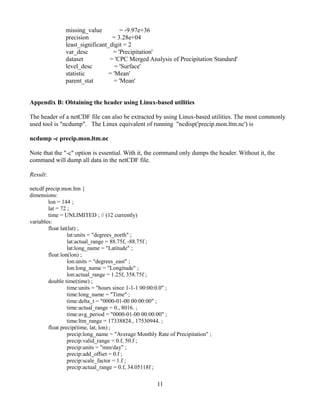
Appendix A. The header of a netCDF file as the output from the example in Step 0
Executing the command, ncdisp('precip.mon.ltm.nc'), would produce the following detailed output
which is the header of the netCDF file, precip.mon.ltm.nc.
Source:
m:small_projectprecip.mon.ltm.nc
Format:
classic
Global Attributes:
Conventions = 'COARDS'
title = 'CPC Merged Analysis of Precipitation (excludes NCEP Reanalysis)'
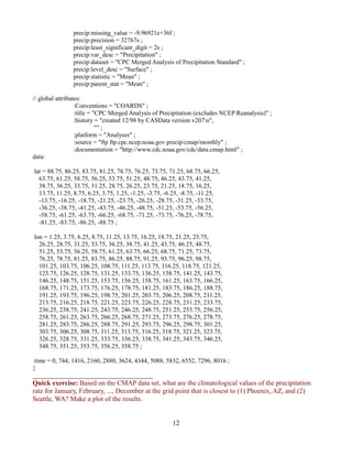
9](https://image.slidesharecdn.com/matlabnetcdfguide-160117203239/85/Matlab-netcdf-guide-9-320.jpg)
![history = 'created 12/98 by CASData version v207
'
platform = 'Analyses'
source = 'ftp ftp.cpc.ncep.noaa.gov precip/cmap/monthly'
documentation = 'http://www.cdc.noaa.gov/cdc/data.cmap.html'
Dimensions:
lon = 144
lat = 72
time = 12 (UNLIMITED)
Variables:
lat
Size: 72x1
Dimensions: lat
Datatype: single
Attributes:
units = 'degrees_north'
actual_range = [8.88e+01 -8.88e+01]
long_name = 'Latitude'
lon
Size: 144x1
Dimensions: lon
Datatype: single
Attributes:
units = 'degrees_east'
long_name = 'Longitude'
actual_range = [1.25e+00 3.59e+02]
time
Size: 12x1
Dimensions: time
Datatype: double
Attributes:
units = 'hours since 1-1-1 00:00:0.0'
long_name = 'Time'
delta_t = '0000-01-00 00:00:00'
actual_range = [0.00e+00 8.02e+03]
avg_period = '0000-01-00 00:00:00'
ltm_range = [1.73e+07 1.75e+07]
precip
Size: 144x72x12
Dimensions: lon,lat,time
Datatype: single
Attributes:
long_name = 'Average Monthly Rate of Precipitation'
valid_range = [0.00e+00 5.00e+01]
units = 'mm/day'
add_offset = 0
scale_factor = 1
actual_range = [0.00e+00 3.41e+01]
10](https://image.slidesharecdn.com/matlabnetcdfguide-160117203239/85/Matlab-netcdf-guide-10-320.jpg)

The document provides a quick guide on how to use Matlab functions to read netCDF files. It explains that a netCDF file contains variable data and header information describing the variables. It then demonstrates various Matlab functions to inspect and extract information from the header, including the number of variables and dimensions, variable names and data types, and dimension lengths. It uses an example netCDF file containing monthly precipitation data to show how to read a single variable, as well as a subsection of a variable, from the file.