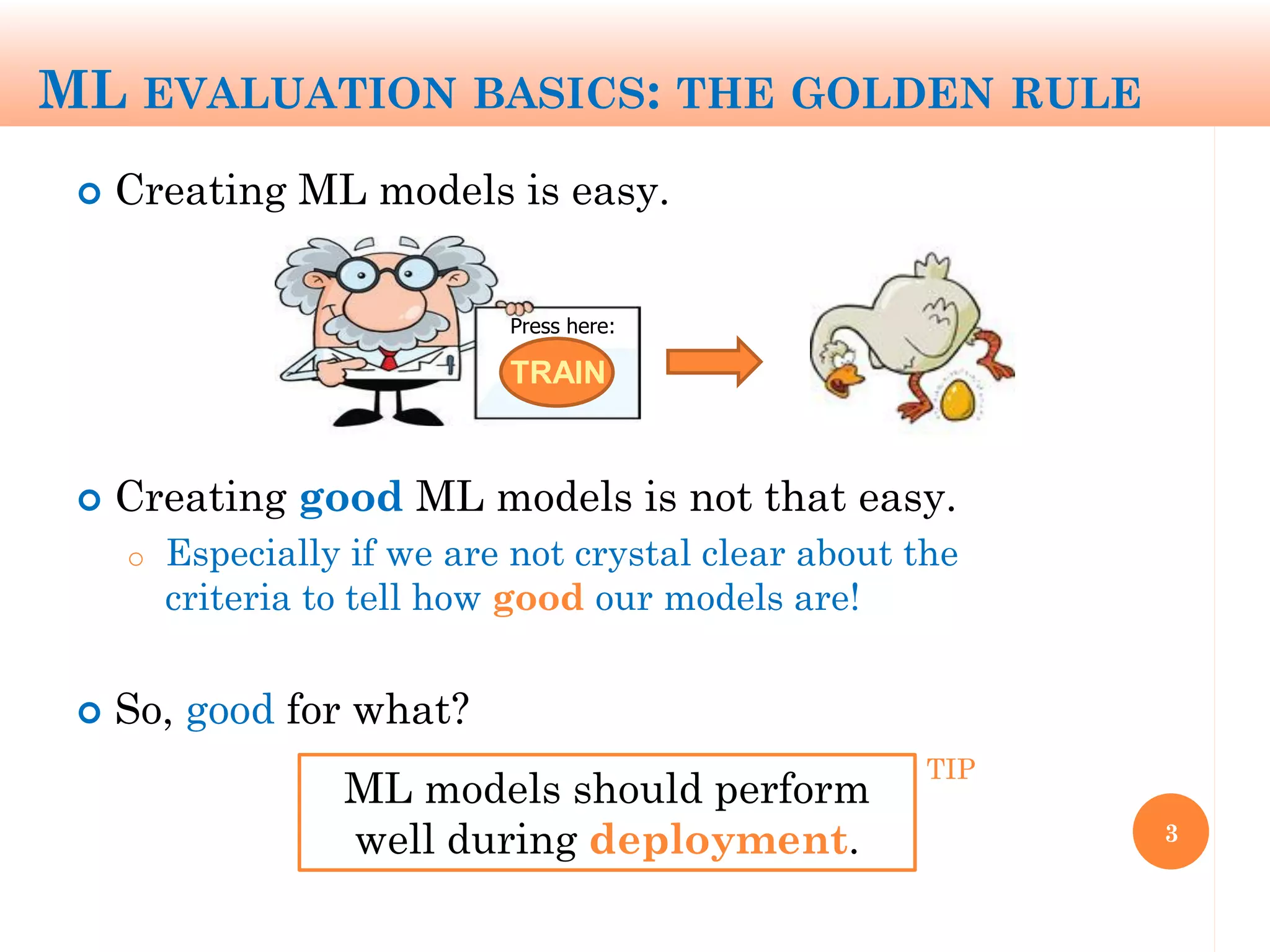
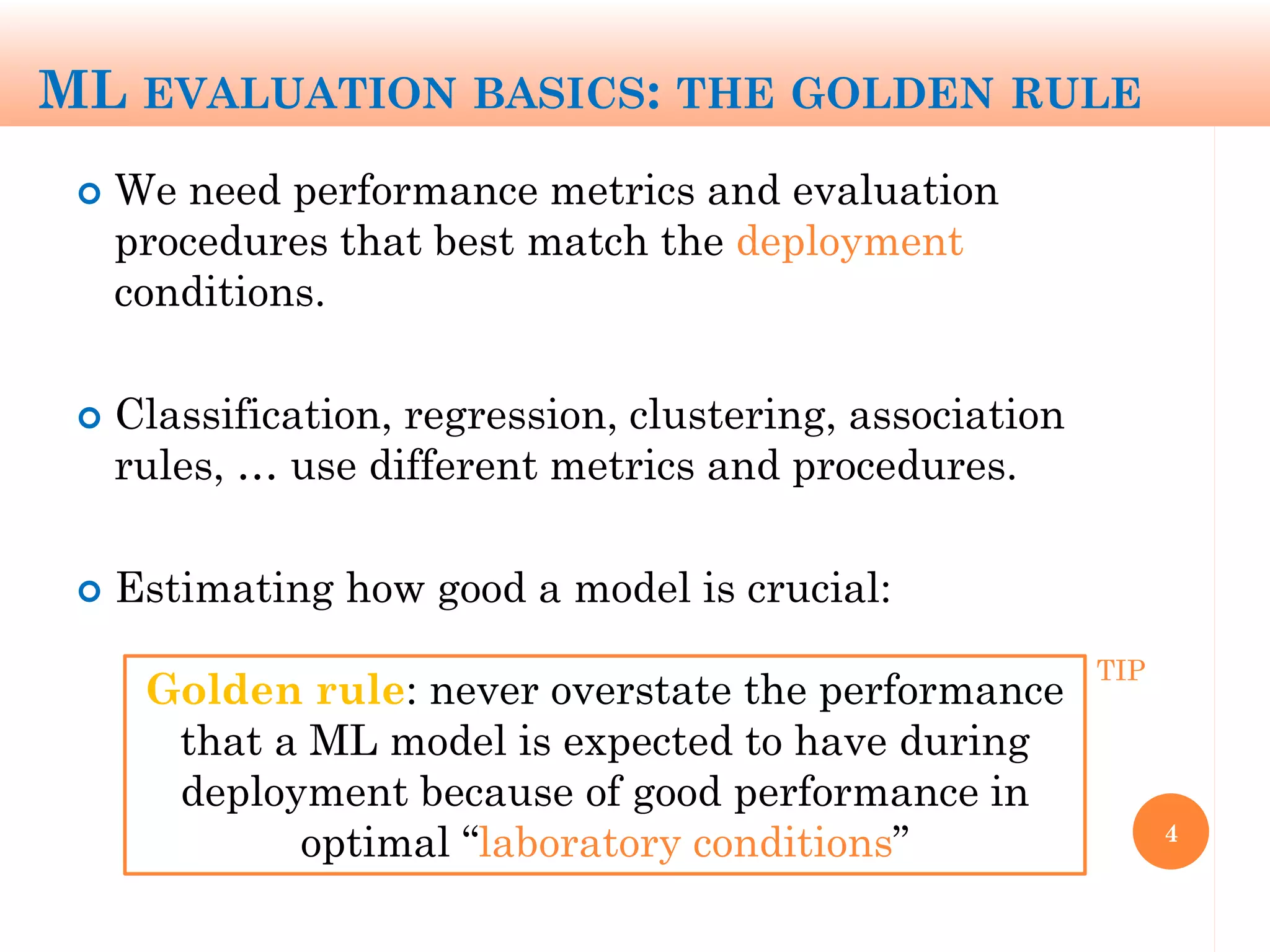
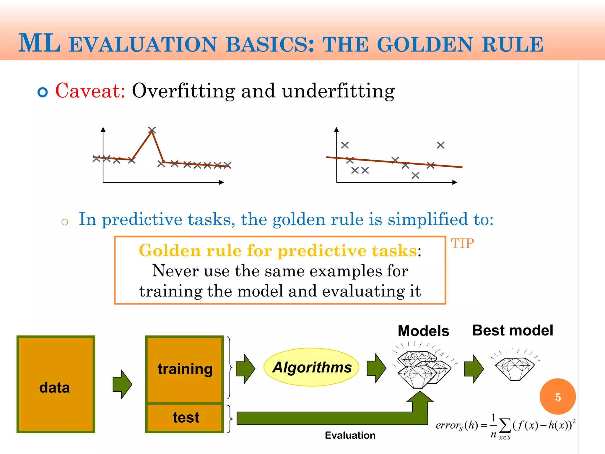
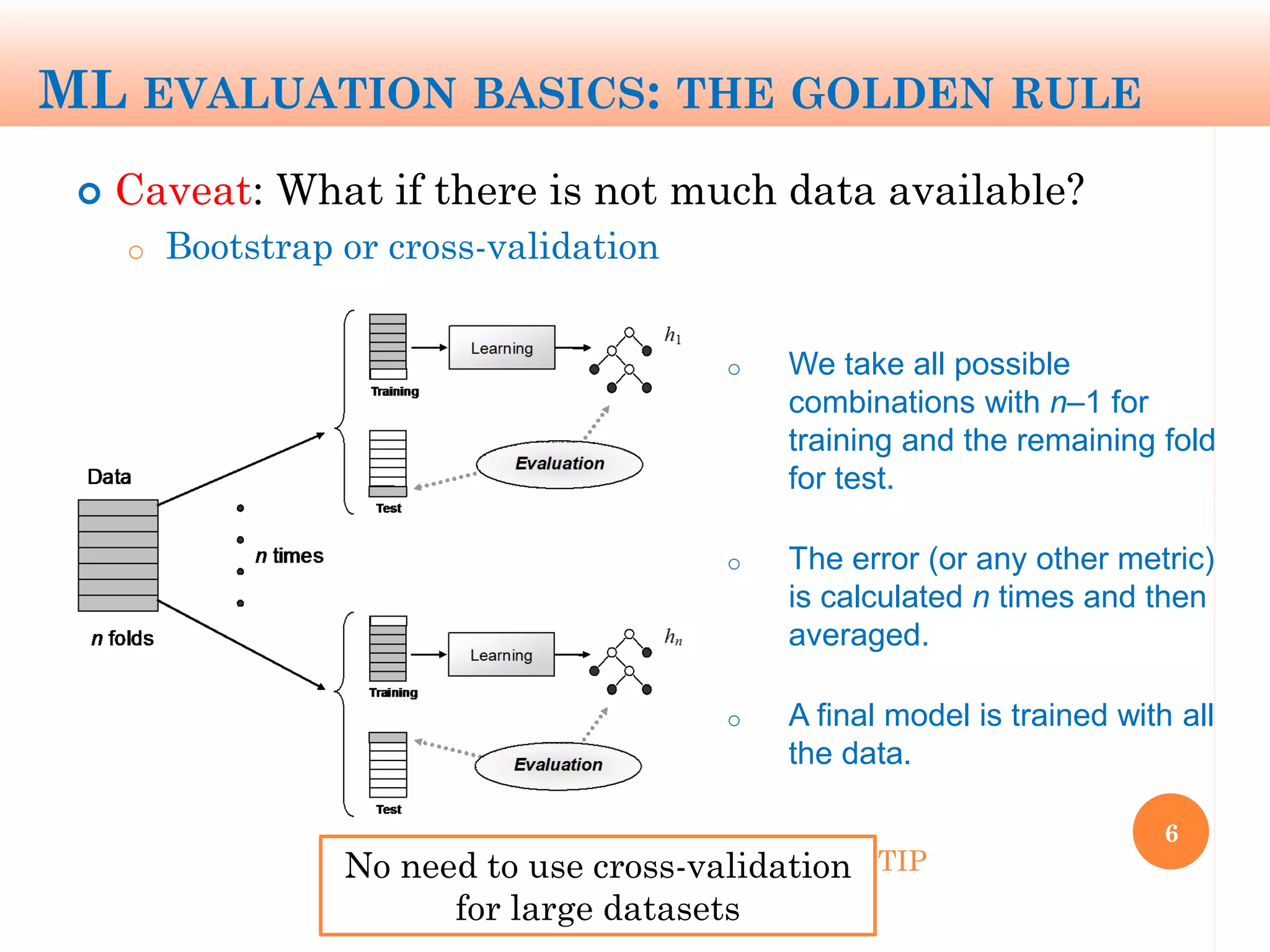
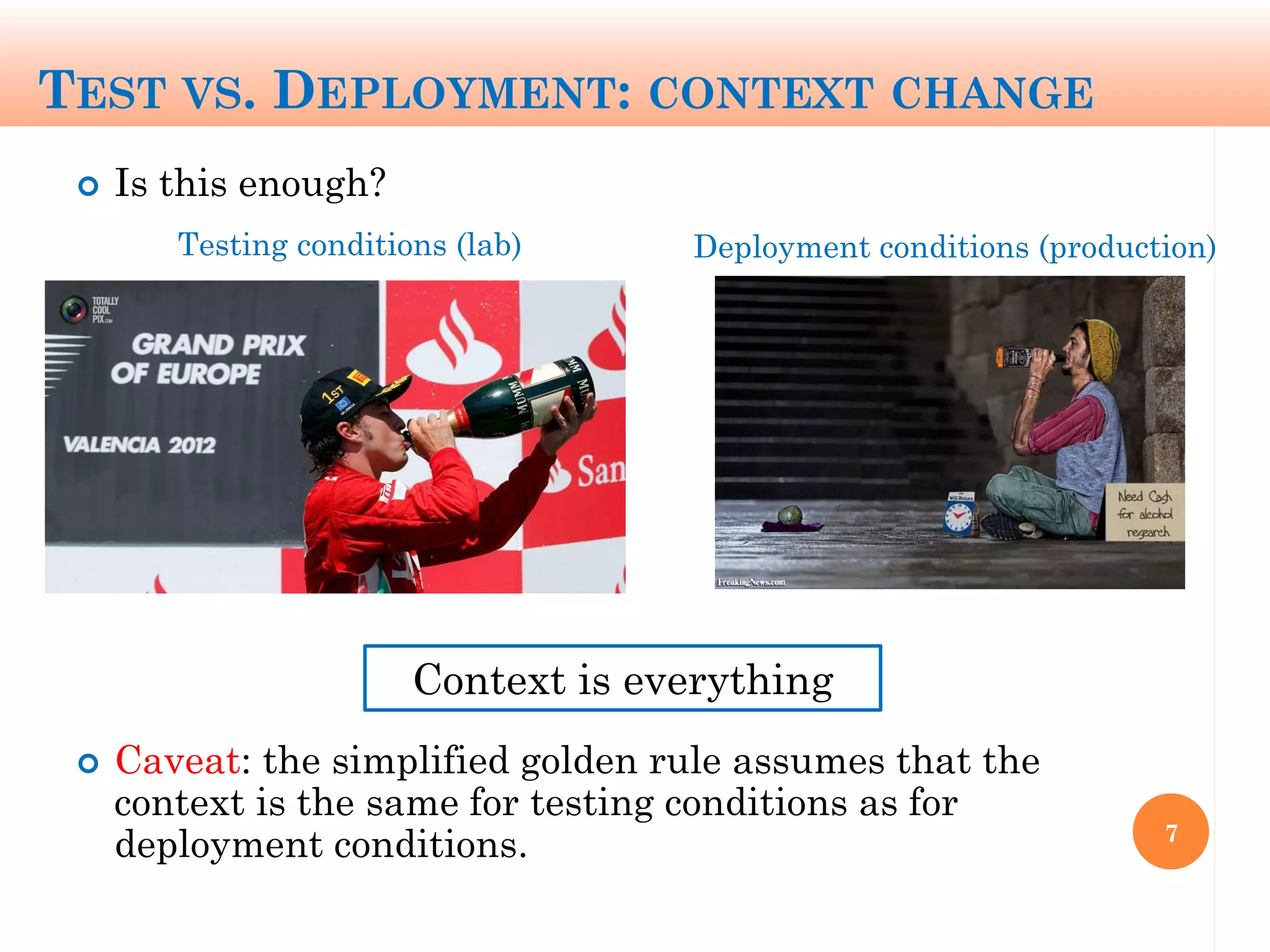
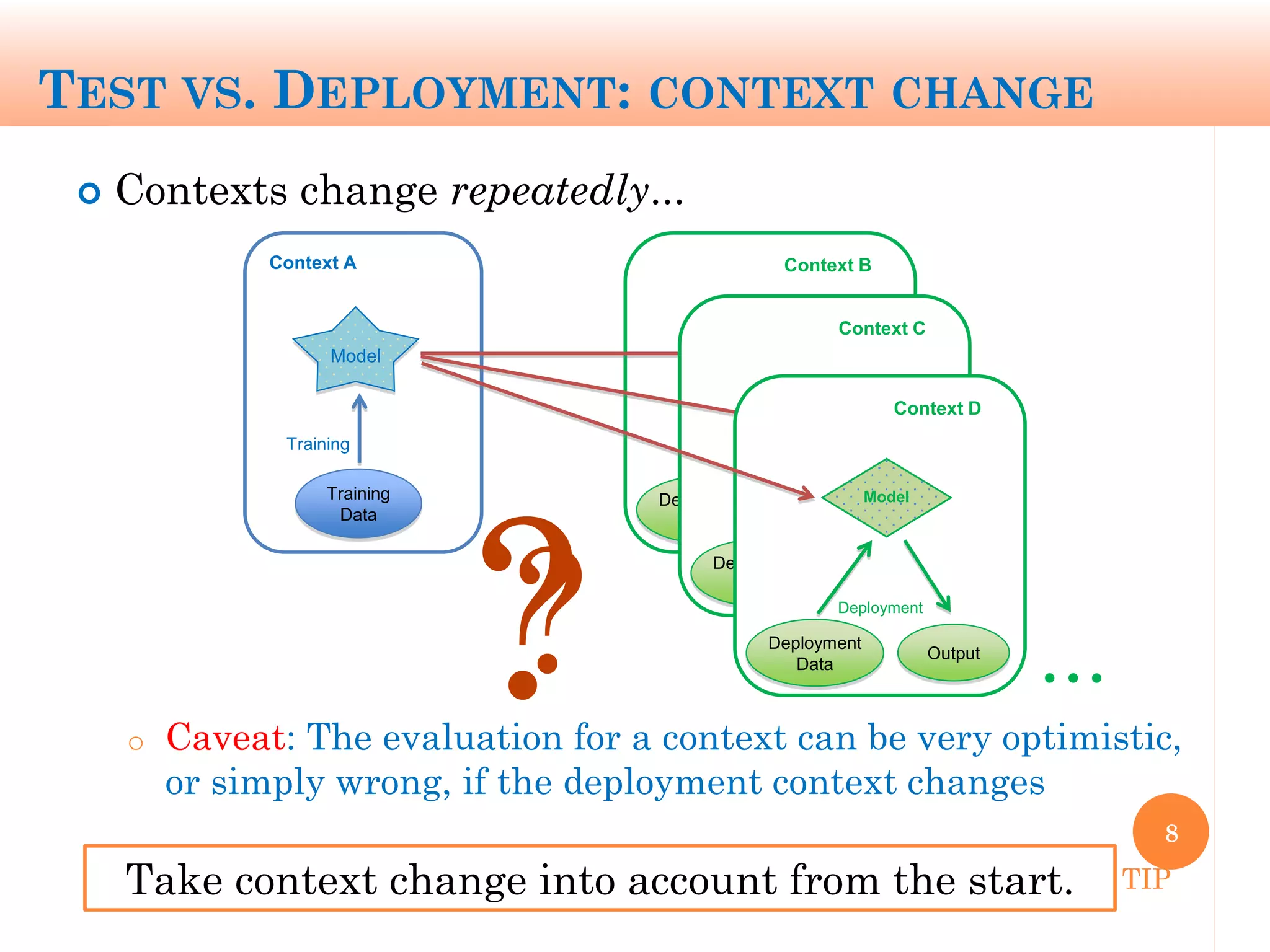
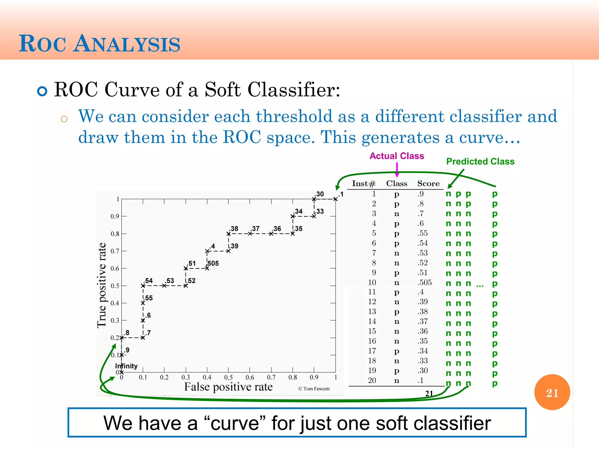
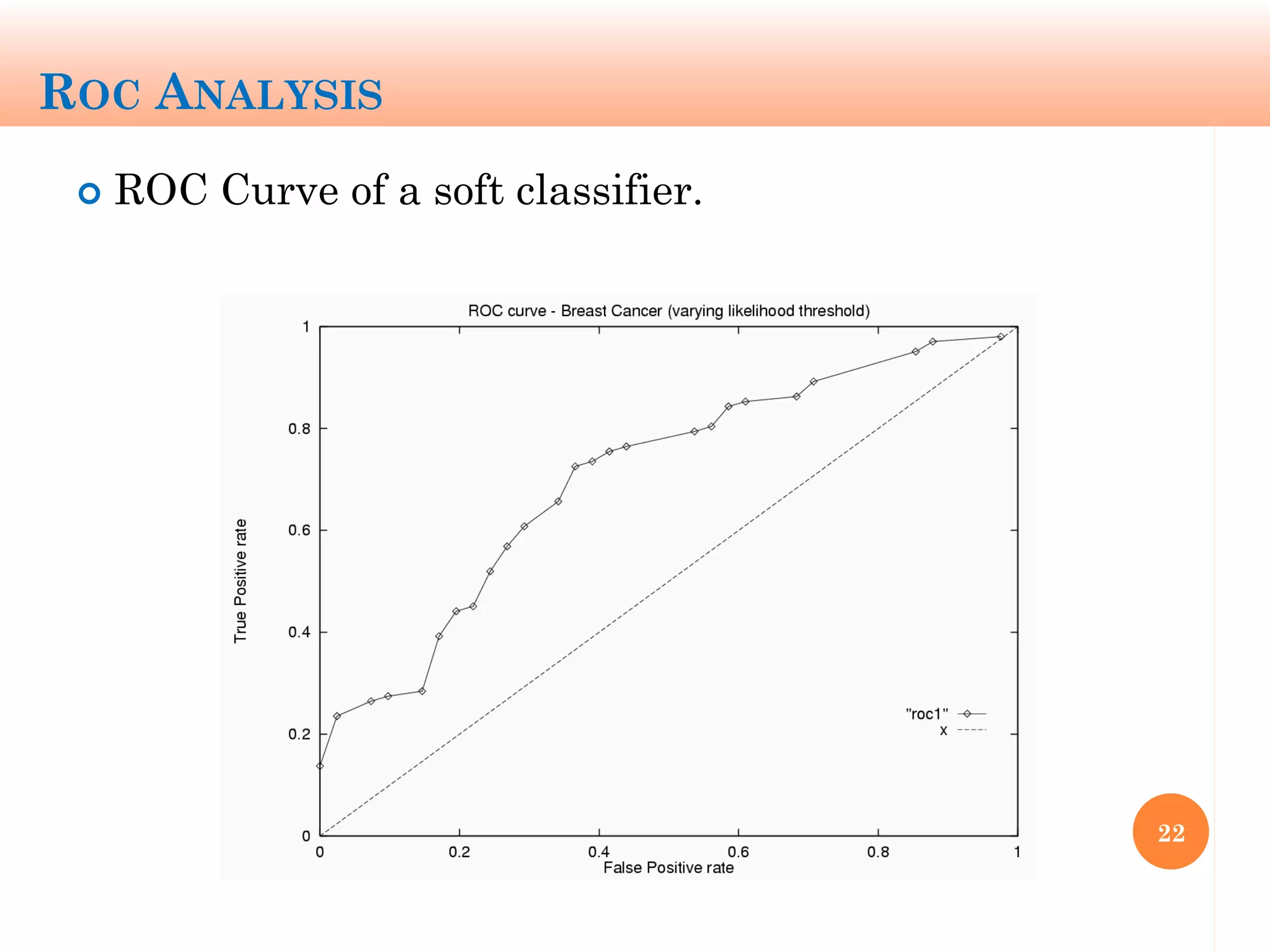
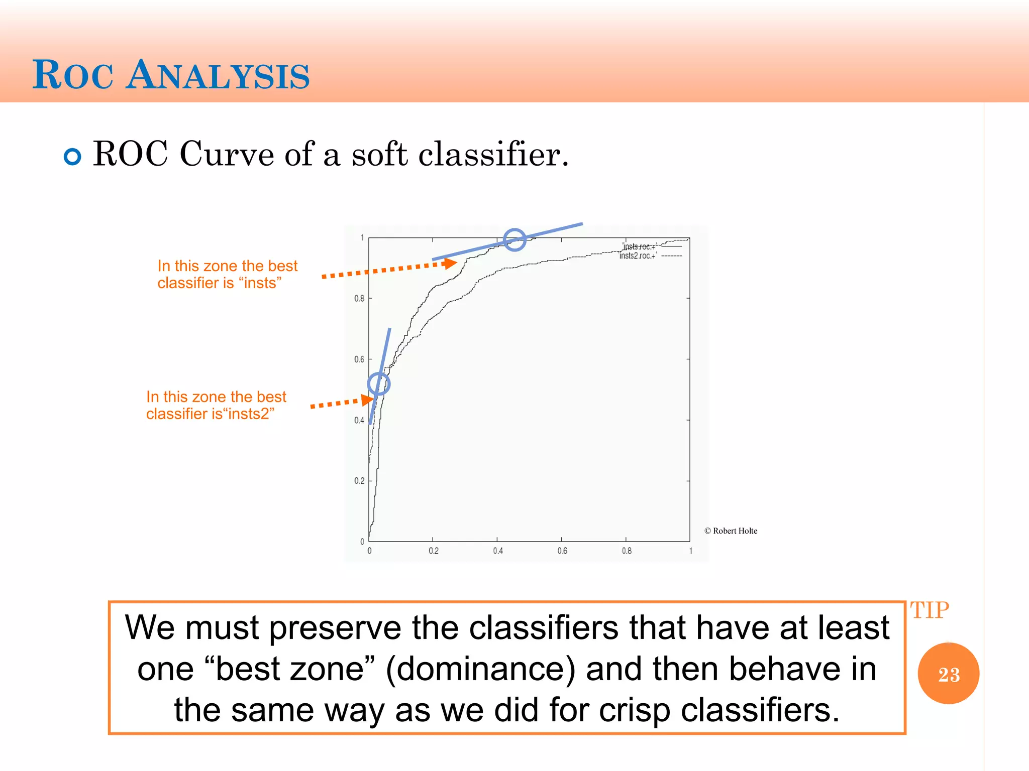
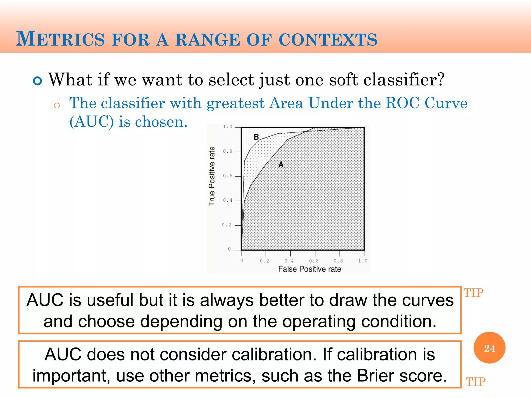
The document discusses machine learning performance evaluation, emphasizing the importance of context and proper measurement metrics for model effectiveness during deployment. It outlines key principles such as avoiding overstatement of model performance due to overfitting, the necessity of considering context changes, and using ROC analysis to assess classifier effectiveness across different conditions. Additionally, it highlights the significance of soft classifiers and the need for cost-sensitive evaluation in complex scenarios, including multiclass and regression problems.

1. MACHINE LEARNING
PERFORMANCE EVALUATION:
TIPS AND PITFALLS
José Hernández-Orallo
DSIC, ETSINF, UPV, jorallo@dsic.upv.es

2. OUTLINE
ML evaluation basics: the golden rule
Test vs. deployment. Context change
Cost and data distribution changes
ROC Analysis
Metrics for a range of contexts
Beyond binary classification
Lessons learnt 2

3. ML EVALUATION BASICS: THE GOLDEN RULE
 Creating ML models is easy.
 Creating good ML models is not that easy.
o Especially if we are not crystal clear about the
criteria to tell how good our models are!
 So, good for what?
3
ML models should perform
well during deployment.
TRAIN
Press here:
TIP

4. ML EVALUATION BASICS: THE GOLDEN RULE
 We need performance metrics and evaluation
procedures that best match the deployment
conditions.
 Classification, regression, clustering, association
rules, … use different metrics and procedures.
 Estimating how good a model is crucial:
4
Golden rule: never overstate the performance
that a ML model is expected to have during
deployment because of good performance in
optimal “laboratory conditions”
TIP

5. ML EVALUATION BASICS: THE GOLDEN RULE
 Caveat: Overfitting and underfitting
o In predictive tasks, the golden rule is simplified to:
5
Golden rule for predictive tasks:
Never use the same examples for
training the model and evaluating it
training
test
Models
Evaluation
Best model


Sx
S xhxf
n
herror 2
))()((
1
)(
data
Algorithms
TIP

6. ML EVALUATION BASICS: THE GOLDEN RULE
 Caveat: What if there is not much data available?
o Bootstrap or cross-validation
6
o We take all possible
combinations with n‒1 for
training and the remaining fold
for test.
o The error (or any other metric)
is calculated n times and then
averaged.
o A final model is trained with all
the data.
No need to use cross-validation
for large datasets
TIP

7. TEST VS. DEPLOYMENT: CONTEXT CHANGE
 Is this enough?
 Caveat: the simplified golden rule assumes that the
context is the same for testing conditions as for
deployment conditions. 7
Context is everything
Testing conditions (lab) Deployment conditions (production)

8. TEST VS. DEPLOYMENT: CONTEXT CHANGE
 Contexts change repeatedly...
o Caveat: The evaluation for a context can be very optimistic,
or simply wrong, if the deployment context changes
8
Context A
Training
Data
Model
Training
Context B
Deployment
Data
Deployment
Output
Model
Context C
Deployment
Data
Deployment
Output
Model Context D
Deployment
Data
Deployment
Output
Model
…??
Take context change into account from the start. TIP

9. TEST VS. DEPLOYMENT: CONTEXT CHANGE
 Types of contexts in ML
o Data shift (covariate, prior probability, concept drift, …).
 Changes in p(X), p(Y), p(X|Y), p(Y|X), p(X,Y)
o Costs and utility functions.
 Cost matrices, loss functions, reject costs, attribute costs, error
tolerance…
o Uncertain, missing or noisy information
 Noise or uncertainty degree, %missing values, missing attribute
set, ...
o Representation change, constraints, background
knowledge.
 Granularity level, complex aggregates, attribute set, etc.
o Task change
 Regression cut-offs, bins, number of classes or clusters,
quantification, …
9

10. COST AND DATA DISTRIBUTION CHANGES
 Classification. Example: 100,000 instances
o High imbalance (π0=Pos/(Pos+Neg)=0.005).
10
10
c1 open close
OPEN 300 500
CLOSE 200 99000
Actual
Pred.
c3 open close
OPEN 400 5400
CLOSE 100 94100
Actual
c2 open close
OPEN 0 0
CLOSE 500 99500
Actual
ERROR: 0,7%
TPR= 300 / 500 = 60%
FNR= 200 / 500 = 40%
TNR= 99000 / 99500 = 99,5%
FPR= 500 / 99500 = 0.5%
PPV= 300 / 800 = 37.5%
NPV= 99000 / 99200 = 99.8%
Macroavg= (60 + 99.5 ) / 2 =
79.75%
ERROR: 0,5%
TPR= 0 / 500 = 0%
FNR= 500 / 500 = 100%
TNR= 99500 / 99500 = 100%
FPR= 0 / 99500 = 0%
PPV= 0 / 0 = UNDEFINED
NPV= 99500 / 10000 = 99.5%
Macroavg= (0 + 100 ) / 2 =
50%
ERROR: 5,5%
TPR= 400 / 500 = 80%
FNR= 100 / 500 = 20%
TNR= 94100 / 99500 = 94.6%
FPR= 5400 / 99500 = 5.4%
PPV= 400 / 5800 = 6.9%
NPV= 94100 / 94200 = 99.9%
Macroavg= (80 + 94.6 ) / 2 =
87.3%
Which classifier is best?
SpecificitySensitivity
Recall
Precision

11. COST AND DATA DISTRIBUTION CHANGES
 Caveat: Not all errors are equal.
o Example: keeping a valve closed in a nuclear plant when
it should be open can provoke an explosion, while opening
a valve when it should be closed can provoke a stop.
o Cost matrix:
11
open close
OPEN 0 100€
CLOSE 2000€ 0
Actual
Predicted
TIP
The best classifier is not the most
accurate, but the one with lowest cost

12. COST AND DATA DISTRIBUTION CHANGES
 Classification. Example: 100,000 instances
o High imbalance (π0=Pos/(Pos+Neg)=0.005).
12
open close
OPEN 0 100€
CLOSE 2000€ 0
Actual
Predicted
c1 open close
OPEN 300 500
CLOSE 200 99000
Actual
Pred
c3 open close
OPEN 400 5400
CLOSE 100 94100
Actual
c2 open close
OPEN 0 0
CLOSE 500 99500
Actual
c1 open close
OPEN 0€ 50,000€
CLOSE 400,000€ 0€
c3 open close
OPEN 0€ 540,000€
CLOSE 200,000€ 0€
c2 open close
OPEN 0€ 0€
CLOSE 1,000,000€ 0€
TOTAL COST: 450,000€ TOTAL COST: 1,000,000€ TOTAL COST: 740,000€
Confusion Matrices
Cost
Matrix
Resulting Matrices
For two classes, the value “slope” (with FNR and FPR)
is sufficient to tell which classifier is best.
This is the operating condition, context or skew.
TIP

13. ROC ANALYSIS
 The context or skew (the class distribution and the
costs of each error) determines classifier goodness.
o Caveat:
 In many circumstances, until deployment time, we do not know
the class distribution and/or it is difficult to estimate the cost
matrix.
 E.g. a spam filter.
 But models are usually learned before.
o SOLUTION:
 ROC (Receiver Operating Characteristic) Analysis.
13

14. ROC ANALYSIS
 The ROC Space
o Using the normalised terms of the confusion matrix:
 TPR, FNR, TNR, FPR:
14
14
ROC Space
0,000
0,200
0,400
0,600
0,800
1,000
0,000 0,200 0,400 0,600 0,800 1,000
False Positives
TruePositives
open close
OPEN 400 12000
CLOSE 100 87500
Actual
Pred
open close
OPEN 0.8 0.121
CLOSE 0.2 0.879
Actual
Pred
TPR= 400 / 500 = 80%
FNR= 100 / 500 = 20%
TNR= 87500 / 99500 = 87.9%
FPR= 12000 / 99500 = 12.1%

15. ROC ANALYSIS
 Good and bad classifiers
15
0 1
1
0
FPR
TPR
• Good classifier.
– High TPR.
– Low FPR.
0 1
1
0
FPR
TPR
0 1
1
0
FPR
TPR
• Bad classifier.
– Low TPR.
– High FPR.
• Bad classifier
(more realistic).

16. ROC ANALYSIS
 The ROC “Curve”: “Continuity”.
16
ROC diagram
0 1
1
0
FPR
TPR
o Given two classifiers:
 We can construct any
“intermediate” classifier just
randomly weighting both
classifiers (giving more or
less weight to one or the
other).
 This creates a “continuum”
of classifiers between any
two classifiers.

17. ROC ANALYSIS
 The ROC “Curve”: Construction
17
ROC diagram
0 1
1
0
FPR
TPR
The diagonal
shows the worst
situation
possible.
We can discard those which are below because
there is no context (combination of class distribution
/ cost matrix) for which they could be optimal.
o Given several classifiers:
 We construct the convex hull of
their points (FPR,TPR) as well as
the two trivial classifiers (0,0) and
(1,1).
 The classifiers below the ROC
curve are discarded.
 The best classifier (from those
remaining) will be selected in
application time…
TIP

18. ROC ANALYSIS
 In the context of application, we choose the optimal
classifier from those kept. Example 1:
18
2
1
FNcost
FPcost

Neg
Pos
 4
22
4 slope
Context (skew):
0%
20%
40%
60%
80%
100%
0% 20% 40% 60% 80% 100%
false positive rate
truepositiverate

19. ROC ANALYSIS
 In the context of application, we choose the optimal
classifier from those kept. Example 2:
19

FPcost
FNcost
 1
8

Neg
Pos
 4

slope  4
8  .5
Context (skew):
0%
20%
40%
60%
80%
100%
0% 20% 40% 60% 80% 100%
false positive rate
truepositiverate

20. ROC ANALYSIS
 Crisp and Soft Classifiers:
o A “hard” or “crisp” classifier predicts a class between a set
of possible classes.
 Caveat: crisp classifiers are not versatile to changing contexts.
o A “soft” or “scoring” (probabilistic) classifier predicts a
class, but accompanies each prediction with an estimation
of the reliability (confidence) of each prediction.
 Most learning methods can be adapted to generate soft classifiers.
o A soft classifier can be converted into a crisp classifier
using a threshold.
 Example: “if score > 0.7 then class A, otherwise class B”.
 With different thresholds, we have different classifiers, giving
more or less relevance to each of the classes
20
Soft or scoring classifiers can be
reframed to each context.
TIP

21. ROC ANALYSIS
 ROC Curve of a Soft Classifier:
o We can consider each threshold as a different classifier and
draw them in the ROC space. This generates a curve…
21
We have a “curve” for just one soft classifier
21
Actual Class
n
n
n
n
n
n
n
n
n
n
n
n
n
n
n
n
n
n
n
n
Predicted Class
p
p
p
p
p
p
p
p
p
p
p
p
p
p
p
p
p
p
p
p
p
n
n
n
n
n
n
n
n
n
n
n
n
n
n
n
n
n
n
n
p
p
n
n
n
n
n
n
n
n
n
n
n
n
n
n
n
n
n
n
...
© Tom Fawcett

22. ROC ANALYSIS
 ROC Curve of a soft classifier.
22

23. ROC ANALYSIS
 ROC Curve of a soft classifier.
23
In this zone the best
classifier is “insts”
In this zone the best
classifier is“insts2”
© Robert Holte
We must preserve the classifiers that have at least
one “best zone” (dominance) and then behave in
the same way as we did for crisp classifiers.
TIP

24. METRICS FOR A RANGE OF CONTEXTS
 What if we want to select just one soft classifier?
o The classifier with greatest Area Under the ROC Curve
(AUC) is chosen.
24
AUC does not consider calibration. If calibration is
important, use other metrics, such as the Brier score. TIP
AUC is useful but it is always better to draw the curves
and choose depending on the operating condition.
TIP

25. BEYOND BINARY CLASSIFICATION
 Cost-sensitive evaluation is perfectly extensible for
classification with more than two classes.
 For regression, we only need a cost function
o For instance, asymmetric absolute error:
25
ERROR actual
low medium high
low 20 0 13
medium 5 15 4predicted
high 4 7 60
COST actual
low medium high
low 0€ 5€ 2€
medium 200€ -2000€ 10€predicted
high 10€ 1€ -15€
Total cost:
-29787€

26. BEYOND BINARY CLASSIFICATION
 ROC analysis for multiclass problems is troublesome.
o Given n classes, there is a n  (n‒1) dimensional space.
o Calculating the convex hull impractical.
 The AUC measure has been extended:
o All-pair extension (Hand & Till 2001).
o There are other extensions.
26
  

c
i
c
ijj
HT jiAUC
cc
AUC
1 ,1
),(
)1(
1

27. BEYOND BINARY CLASSIFICATION
 ROC analysis for regression (using shifts).
o The operating condition is the asymmetry factor α. For
instance if α=2/3 means that underpredictions are twice
as expensive than overpredictions.
o The area over the curve (AOC) is the error variance. If
the model is unbiased, then it is ½ MSE.
27

28. LESSONS LEARNT
 Model evaluation goes much beyond split or cross-
validation + metric (accuracy or MSE).
 Models can be generated once but then applied to
different contexts / operating conditions.
 Drawing models for different operating conditions
allow us to determine dominance regions and the
optimal threshold to make optimal decisions.
 Soft (scoring) models are much more powerful than
crisp models. ROC analysis really makes sense for
soft models.
 Areas under/over the curves are an aggregate of the
performance on a range of operating conditions, but
should not replace ROC analysis. 28

29. LESSONS LEARNT
 We have just seen an example with one kind of
context change: cost changes and output distribution.
 Similar approaches exist with other types of context
changes
o Uncertain, missing or noisy information
o Representation change, constraints, background
knowledge.
o Task change
29
 http://www.reframe-d2k.org/