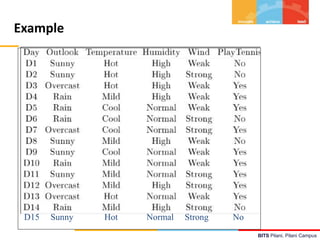
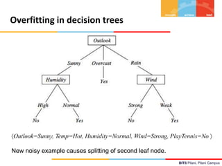
This document contains lecture notes from BITS Pilani on machine learning and decision trees. It discusses decision trees, information gain, entropy, overfitting, and techniques for handling continuous values and missing data in decision trees. The key topics covered are decision tree induction using the ID3 algorithm, measures of information like entropy used for splitting nodes, and methods for avoiding overfitting like reduced error pruning and converting decision trees to rules for post-pruning.

1. BITS Pilani
Pilani Campus
Machine Learning
ZG565
Dr. Sugata Ghosal
sugata.ghosal@pilani.bits-pilani.ac.in

2. BITS Pilani, Pilani Campus
BITS Pilani
Pilani Campus
LectureNo.–7|DecisionTree
Date–01/07/2023
Time:2PM–4PM

3. BITS Pilani, Pilani Campus
Session Content
3
• Decision Tree
• Handling overfitting
• Continuous values
• Missing Values

4. BITS Pilani, Pilani Campus
Decision trees
 Decision Trees is one of the most widely used
and practical methods of classification
 Method for approximating discrete-valued
functions
 Learned functions are represented as decision
trees (or if-then-else rules)
 Expressive hypotheses space

5. BITS Pilani, Pilani Campus
Decision Tree
• Advantages:
– Inexpensive to construct
– Extremely fast at classifying unknown records
– Easy to interpret for small-sized trees
– Can easily handle redundant or irrelevant attributes (unless
the attributes are interacting)
• Disadvantages:
– Space of possible decision trees is exponentially large.
Greedy approaches are often unable to find the best tree.
– Does not take into account interactions between attributes
– Each decision boundary involves only a single attribute
5

6. BITS Pilani, Pilani Campus
6
Outlook=Sunny, Temp=Hot, Humidity=High, Wind=Strong No
Decision tree representation (PlayTennis)

7. BITS Pilani, Pilani Campus
Decision trees expressivity
• Decision trees represent a disjunction of conjunctions on constraints on the
value of attributes:
(Outlook = Sunny  Humidity = Normal) 
(Outlook = Overcast) 
(Outlook = Rain  Wind = Weak)

8. BITS Pilani, Pilani Campus
Measure of Information
20 March 2024
• The amount of information (surprise element)
conveyed by a message is inversely proportional to its
probability of occurrence. That is
• The mathematical operator satisfies above
properties is the logarithmic operator.
1
k
k
I
p

1
log
k r
k
I units
p


9. BITS Pilani, Pilani Campus
Entropy
• Entropy of discrete random variable X={x1, x2…xn}
; since: log2(1/P(event))= -log2P(event)
• As uncertainty increases, entropy increases
• Entropy across all values

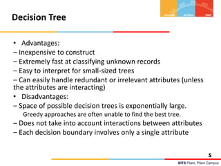
10. BITS Pilani, Pilani Campus
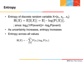
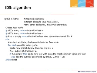
Entropy in general
• Entropy measures the amount of information in
a random variable
H(X) = – p+ log2 p+ – p– log2 p– X = {+, –}
for binary classification [two-valued random variable]
c c
H(X) = –  pi log2 pi =  pi log2 1/ pi X = {i, …, c}
i=1 i=1
for classification in c classes

11. BITS Pilani, Pilani Campus
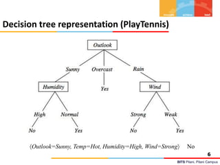
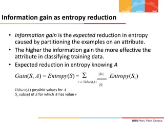
Entropy in binary classification
• Entropy measures the impurity of a collection of
examples. It depends from the distribution of the
random variable p.
– S is a collection of training examples
– p+ the proportion of positive examples in S
– p– the proportion of negative examples in S
Entropy (S)  – p+ log2 p+ – p–log2 p– [0 log20 = 0]
Entropy ([14+, 0–]) = – 14/14 log2 (14/14) – 0 log2 (0) = 0
Entropy ([9+, 5–]) = – 9/14 log2 (9/14) – 5/14 log2 (5/14) = 0.94
Entropy ([7+, 7– ]) = – 7/14 log2 (7/14) – 7/14 log2 (7/14) =
= 1/2 + 1/2 = 1 [log21/2 = – 1]
Note: the log of a number < 1 is negative, 0  p  1, 0  entropy  1
• https://www.easycalculation.com/log-base2-calculator.php

12. BITS Pilani, Pilani Campus
Information gain as entropy reduction
• Information gain is the expected reduction in entropy
caused by partitioning the examples on an attribute.
• The higher the information gain the more effective the
attribute in classifying training data.
• Expected reduction in entropy knowing A
Gain(S, A) = Entropy(S) −  Entropy(Sv)
v  Values(A)
Values(A) possible values for A
Sv subset of S for which A has value v
|Sv|
|S|

13. BITS Pilani, Pilani Campus
Example

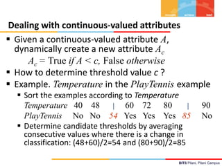
14. BITS Pilani, Pilani Campus
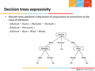
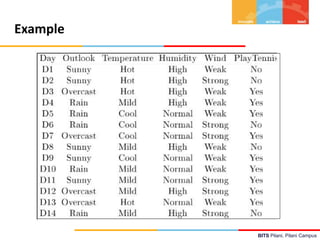
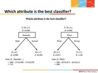
Example: Information gain
• Let
– Values(Wind) = {Weak, Strong}
– S = [9+, 5−]
– SWeak = [6+, 2−]
– SStrong = [3+, 3−]
• Information gain due to knowing Wind:
Gain(S, Wind) = Entropy(S) − 8/14 Entropy(SWeak) − 6/14 Entropy(SStrong)
= 0.94 − 8/14  0.811 − 6/14  1.00
= 0.048

15. BITS Pilani, Pilani Campus
Example

16. BITS Pilani, Pilani Campus
Which attribute is the best classifier?

17. BITS Pilani, Pilani Campus
First step: which attribute to test at the root?
 Which attribute should be tested at the root?
 Gain(S, Outlook) = 0.246
 Gain(S, Humidity) = 0.151
 Gain(S, Wind) = 0.084
 Gain(S, Temperature) = 0.029
 Outlook provides the best prediction for the
target
 Lets grow the tree:
 add to the tree a successor for each possible value of
Outlook
 partition the training samples according to the value
of Outlook

18. BITS Pilani, Pilani Campus
After first step

19. BITS Pilani, Pilani Campus
Second step
 Working on Outlook=Sunny node:
Gain(SSunny, Humidity) = 0.970  3/5  0.0  2/5  0.0 = 0.970
Gain(SSunny, Wind) = 0.970  2/5  1.0  3.5  0.918 = 0 .019
Gain(SSunny, Temp.) = 0.970  2/5  0.0  2/5  1.0  1/5  0.0 =
0.570
 Humidity provides the best prediction for the target
 Lets grow the tree:
 add to the tree a successor for each possible value of Humidity
 partition the training samples according to the value of
Humidity

20. BITS Pilani, Pilani Campus
Second and third steps
{D1, D2, D8}
No
{D9, D11}
Yes
{D4, D5, D10}
Yes
{D6, D14}
No

21. BITS Pilani, Pilani Campus
ID3: algorithm
ID3(X, T, Attrs) X: training examples:
T: target attribute (e.g. PlayTennis),
Attrs: other attributes, initially all attributes
Create Root node
If all X's are +, return Root with class +
If all X's are –, return Root with class –
If Attrs is empty return Root with class most common value of T in X
else
A  best attribute; decision attribute for Root  A
For each possible value vi of A:
- add a new branch below Root, for test A = vi
- Xi  subset of X with A = vi
- If Xi is empty then add a new leaf with class the most common value of T in X
else add the subtree generated by ID3(Xi, T, Attrs  {A})
return Root

22. BITS Pilani, Pilani Campus
Prefer shorter hypotheses: Occam's razor
 Why prefer shorter hypotheses?
 Arguments in favor:
 There are fewer short hypotheses than long ones
 If a short hypothesis fits data unlikely to be a
coincidence
 Elegance and aesthetics
 Arguments against:
 Not every short hypothesis is a reasonable one.
 Occam's razor says that when presented with
competing hypotheses that make the same
predictions, one should select the solution which
is simple"

23. BITS Pilani, Pilani Campus
Issues in decision trees learning
 Overfitting
 Reduced error pruning
 Rule post-pruning
 Extensions
 Continuous valued attributes
 Handling training examples with missing attribute
values

24. BITS Pilani, Pilani Campus
Overfitting: definition
• overfitting is "the production of an analysis that
corresponds too closely or exactly to a particular
set of data
• Building trees that “adapt too much” to the
training examples may lead to “overfitting”.
• May therefore fail to fit additional data or predict
future observations reliably
• overfitted model is a statistical model that
contains more parameters than can be justified
by the data

25. BITS Pilani, Pilani Campus
Example
D15 Sunny Hot Normal Strong No

26. BITS Pilani, Pilani Campus
Overfitting in decision trees
Outlook=Sunny, Temp=Hot, Humidity=Normal, Wind=Strong, PlayTennis=No 
New noisy example causes splitting of second leaf node.

27. BITS Pilani, Pilani Campus
Avoid overfitting in Decision Trees
 Two strategies:
1. Stop growing the tree earlier the tree, before
perfect classification
2. Allow the tree to overfit the data, and then post-
prune the tree
 Training and validation set
 split the training in two parts (training and
validation) and use validation to assess the utility
of post-pruning
 Reduced error pruning
 Rule post pruning

28. BITS Pilani, Pilani Campus
Reduced-error pruning
 Each node is a candidate for pruning
 Pruning consists in removing a subtree rooted in
a node: the node becomes a leaf and is assigned
the most common classification
 Nodes are removed only if the resulting tree
performs no worse on the validation set.
 Nodes are pruned iteratively: at each iteration
the node whose removal most increases
accuracy on the validation set is pruned.
 Pruning stops when no pruning increases
accuracy

29. BITS Pilani, Pilani Campus
Rule post-pruning
1. Create the decision tree from the training set
2. Convert the tree into an equivalent set of rules
– Each path corresponds to a rule
– Each node along a path corresponds to a pre-condition
– Each leaf classification to the post-condition
3. Prune (generalize) each rule by removing those
preconditions whose removal improves accuracy …
– … over validation set
4. Sort the rules in estimated order of accuracy, and
consider them in sequence when classifying new
instances

30. BITS Pilani, Pilani Campus
Converting to rules
(Outlook=Sunny)(Humidity=High) ⇒ (PlayTennis=No)

31. BITS Pilani, Pilani Campus
Rule Post-Pruning
• Convert tree to rules (one for each path from
root to a leaf)
• For each antecedent in a rule, remove it if
error rate on validation set does not decrease
• Sort final rule set by accuracy
Outlook=sunny ^ humidity=high -> No
Outlook=sunny ^ humidity=normal -> Yes
Outlook=overcast -> Yes
Outlook=rain ^ wind=strong -> No
Outlook=rain ^ wind=weak -> Yes
Compare first rule to:
Outlook=sunny->No
Humidity=high->No
Calculate accuracy of 3 rules
based on validation set and
pick best version.

32. BITS Pilani, Pilani Campus
Why converting to rules?
 Each distinct path produces a different rule: a
condition removal may be based on a local
(contextual) criterion. Node pruning is global and
affects all the rules
 Provides flexibility of not removing entire node
 In rule form, tests are not ordered and there is no
book-keeping involved when conditions (nodes)
are removed
 Converting to rules improves readability for
humans

33. BITS Pilani, Pilani Campus
Dealing with continuous-valued attributes
 Given a continuous-valued attribute A,
dynamically create a new attribute Ac
Ac = True if A < c, False otherwise
 How to determine threshold value c ?
 Example. Temperature in the PlayTennis example
 Sort the examples according to Temperature
Temperature 40 48 | 60 72 80 | 90
PlayTennis No No 54 Yes Yes Yes 85 No
 Determine candidate thresholds by averaging
consecutive values where there is a change in
classification: (48+60)/2=54 and (80+90)/2=85

34. BITS Pilani, Pilani Campus
Problems with information gain
• Natural bias of information gain: it favors attributes
with many possible values.
• Consider the attribute Date in the PlayTennis example.
– Date would have the highest information gain since it
perfectly separates the training data.
– It would be selected at the root resulting in a very broad
tree
– Very good on the training, this tree would perform poorly
in predicting unknown instances. Overfitting.
• The problem is that the partition is too specific, too
many small classes are generated.
• We need to look at alternative measures …

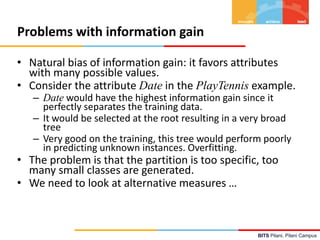
35. BITS Pilani, Pilani Campus
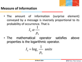
An alternative measure: gain ratio
c |Si | |Si |
SplitInformation(S, A)  −  log2
i=1 |S | |S |
• Si are the sets obtained by partitioning on value i of A
• SplitInformation measures the entropy of S with respect to the values of A.
The more uniformly dispersed the data the higher it is.
Gain(S, A)
GainRatio(S, A) 
SplitInformation(S, A)
• GainRatio penalizes attributes that split examples in many small classes such
as Date. Let |S |=n, Date splits examples in n classes
– SplitInformation(S, Date)= −[(1/n log2 1/n)+…+ (1/n log2 1/n)]= −log21/n =log2n
• Compare with A, which splits data in two even classes:
– SplitInformation(S, A)= − [(1/2 log21/2)+ (1/2 log21/2) ]= − [− 1/2 −1/2]=1

36. BITS Pilani, Pilani Campus
Handling missing values training
data
 How to cope with the problem that the value
of some attribute may be missing?
 The strategy: use other examples to guess
attribute
1. Assign the value that is most common among the
training examples at the node
2. Assign a probability to each value, based on
frequencies, and assign values to missing
attribute, according to this probability
distribution

37. BITS Pilani, Pilani Campus
Applications
Suited for following classification problems:
• Applications whose Instances are represented by attribute-
value pairs.
• The target function has discrete output values
• Disjunctive descriptions may be required
• The training data may contain missing attribute values
Real world applications
• Biomedical applications
• Manufacturing
• Banking sector
• Make-Buy decisions

38. BITS Pilani, Pilani Campus
Good References
Decision Tree
• https://www.youtube.com/watch?v=eKD5gxPPeY0
&list=PLBv09BD7ez_4temBw7vLA19p3tdQH6FYO&i
ndex=1
Overfitting
• https://www.youtube.com/watch?time_continue=
1&v=t56Nid85Thg
• https://www.youtube.com/watch?v=y6SpA2Wuyt8
Random Forest
• https://www.stat.berkeley.edu/~breiman/RandomF
orests/