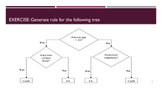
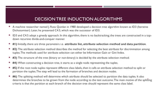
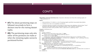
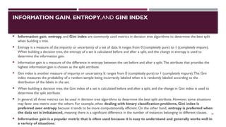
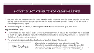
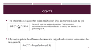
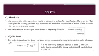
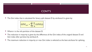
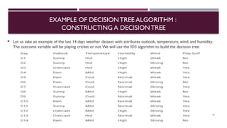
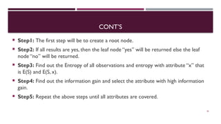
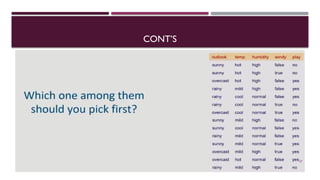
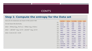
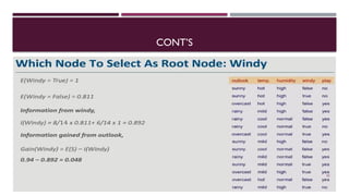
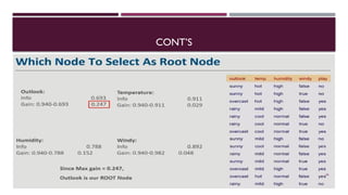
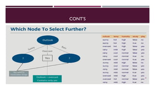
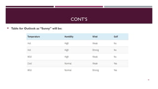
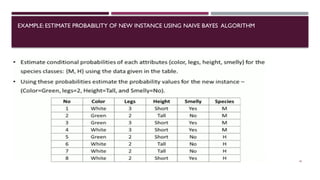
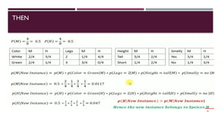
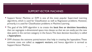
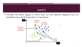
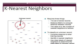
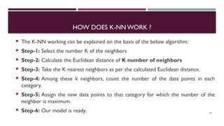
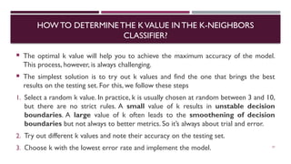
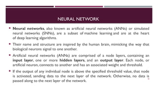
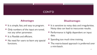
Chapter 3 discusses classification and prediction in machine learning, defining classification as the categorization of data into classes based on labeled data for training. It covers various classification methods including decision trees, Bayesian classification, and support vector machines, highlighting the importance of classifier accuracy and data preprocessing. The document also elaborates on the processes involved in building classifiers, the use of metrics like information gain and Gini index for attribute selection, and provides examples of practical applications of classification.

1. CHAPTER 3
Classification and Prediction
1

2. CONTENTS
3.1What is classification? What is prediction?
3.2 Issues regarding classification and
prediction
3.3 Classification by decision tree induction
3.4 Bayesian classification
3.5 Support vector machines
3.6 Classification by back propagation
3.7 Other classification methods
3.7.1 K-nearest neighbor classifier
3.7.2 Neural Network
3.7.3 Genetic algorithm
3.8 Prediction
3.9 Classifier accuracy
2

3. WHAT IS CLASSIFICATION?
 Classification is the process of categorizing given set of data /structured, unstructured/ in to classes.
 It is part of supervised machine learning in which we put labeled data for training.
 It is a type of supervised learning technique where an algorithm is trained on a labeled dataset to predict the
class or category of new, unseen data.
 The main objective of classification machine learning is to build a model that can accurately assign a label or
category to a new observation based on its features.
 For example, a classification model might be trained on a dataset of images labeled as either bird or animal and
then used to predict the class of new, unseen images of birds or animals based on their features such as color,
texture, and shape.
 Categorized classes are named as categories, target, or label.
 The process starts with predicting the classes of given data points.
3

4. WHAT IS PREDICTION?
 The practice of using data to create predictions or foresee future events is known as machine
learning prediction.
 Machine learning prediction, or prediction in machine learning, refers to the output of an algorithm
that has been trained on a historical dataset.
 The algorithm then generates probable values for unknown variables in each record of the new data.
 The purpose of prediction in machine learning is to project a probable data set that relates back to
the original data. Or
 Building models that can recognize patterns in data and utilize those patterns to create precise
predictions about novel, unforeseen data is the aim of machine learning prediction.
4

5. EXAMPLE
 A bank loans officer needs analysis of her data in order to learn which loan applicants are safe
―
and which are risky for the bank.
―
 A marketing manager at All Electronics needs data analysis to
help guess whether a customer with a given profile will buy a new computer.
 A medical researcher wants to analyse breast cancer data in order to predict which one of three
specific treatments a patient should receive.
 In each of these examples, the data analysis task is classification, where a model or classifier is
constructed to predict categorical labels, such as safe or risky for the loan application data; yes or
no for the marketing data; or treatment A, treatment B, or treatment C for the medical data.
 These categories can be represented by discrete values, where the ordering among values has no
meaning. For example, the values 1, 2, and 3 may be used to represent treatments A, B, and C, where
there is no ordering implied among this group of treatment regimes. 5

6. CONT’S
 Suppose that the marketing manager would like to predict how much a given
customer will spend during a sale at All Electronics.
 This data analysis task is an example of numeric prediction, where
the model constructed predicts a continuous valued function, or ordered value, as
opposed to a categorical label.This model is a predictor.
 Data classification is a two-step process.
A. Building the Classifier or Model
B. Using Classifier for Classification
6

7. CONT’S
A. Building the Classifier or Model
 This step is the learning step or the learning
phase.
 In this step the classification algorithms build
the classifier.
 The classifier is built from the training set made
up of database tuples and their associated class
labels.
 Each tuple that constitutes the training set is
referred to as a category or class
7

8. CONT’S
B. Using Classifier for Classification
 In this step, the classifier is used for
classification.
 Here the test data is used to estimate the
accuracy of classification rules.
 The classification rules can be applied to the
new data tuples if the accuracy is considered
acceptable
8

9. CONT’S
9
 The general approach for building classification models is given below:

10. ISSUES REGARDING CLASSIFICATION AND PREDICTION
 Data cleaning:This refers to the preprocessing of data in order to remove or reduce
noise (by applying smoothing techniques, for example) and the treatment of missing
values (e.g., by replacing a missing value with the most commonly occurring value for
that attribute, or with the most probable value based on statistics).
 Relevance analysis: Many of the attributes in the data may be redundant. Correlation
analysis can be used to identify whether any two given attributes are statistically related.
 Data transformation and reduction: The data may be transformed by
normalization, Normalization involves scaling all values for a given attribute so that they
fall within a small specified range, such as -1.0 to 1.0, or 0.0 to 1.0. In methods that use
distance measurements, for example, this would prevent attributes with initially large
ranges (like, say, income) from out weighing attributes with initially smaller ranges (such
as binary attributes).
10

11. CLASSIFICATION BY DECISION TREE INDUCTION
 Classification is a two-step process, learning step and prediction step, in machine learning.
 In the learning step, the model is developed based on given training data. In the prediction step, the
model is used to predict the response for given data.
 Decision Tree is one of the easiest and popular classification algorithms to understand and interpret.
 Decision tree induction is the learning of decision trees from class -labeled training tuples.
 A decision tree is a flowchart-like tree structure, where each internal node (non-leaf node) denotes a
test on an attribute, each branch represents an outcome of the test, and each leaf node (or terminal
node) holds a class label.The topmost node in a tree is the root node.
11

12. NODES IN DECISIONTREE
 Root Node
 Internal Node/Branch Node
 Leaf Node
12

13. CONT’S
 In supervised learning, the target result is already known. Decision trees can be used for both
categorical and numerical data.The categorical data represent gender, marital status, etc. while the
numerical data represent age, temperature, etc.
13

14. DECISION TREE RULE GENERATION
From above decision tree we have two construct five rules.
Rule 1: If outlook is sunny and windy is false, playgof is “Yes”
Rule 2: If outllok is sunny and windy is true, playgolf is “No”.
…
.
.
.
Rule 5.
14

15. THE BENEFITS OF HAVING A DECISIONTREE ARE AS FOLLOWS −
 Decision Trees usually mimic human thinking ability while making a decision, so it is easy
to understand.
 The logic behind the decision tree can be easily understood because it shows a tree-like
structure.
 It does not require any domain knowledge.
 The learning and classification steps of a decision tree are simple and fast
15

16. DECISION TREE INDUCTION ALGORITHMS
 ID3 (Iterative Dichotomiser).
 C4.5, which was the successor of ID3.
16

17. EXERCISE: Generate rule for the following tree
17

18. DECISION TREE INDUCTION ALGORITHMS
 A machine researcher named J. Ross Quinlan in 1980 developed a decision tree algorithm known as ID3 (Iterative
Dichotomiser). Later, he presented C4.5, which was the successor of ID3.
 ID3 and C4.5 adopt a greedy approach. In this algorithm, there is no backtracking; the trees are constructed in a top-
down recursive divide-and-conquer manner.
 #1) Initially, there are three parameters i.e. attribute list, attribute selection method and data partition.
 #2) The attribute selection method describes the method for selecting the best attribute for discrimination among
tuples.The methods used for attribute selection can either be Information Gain or Gini Index.
 #3) The structure of the tree (binary or non-binary) is decided by the attribute selection method.
 #4) When constructing a decision tree, it starts as a single node representing the tuples.
 #5) If the root node tuples represent different class labels, then it calls an attribute selection method to split or
partition the tuples.The step will lead to the formation of branches and decision nodes.
 #6) The splitting method will determine which attribute should be selected to partition the data tuples. It also
determines the branches to be grown from the node according to the test outcome.The main motive of the splitting
criteria is that the partition at each branch of the decision tree should represent the same class label.
18

19. CONT’S
 #7) The above partitioning steps are
followed recursively to form a
decision tree for the training dataset
tuples.
 #8) The partitioning stops only when
either all the partitions are made or
when the remaining tuples cannot be
partitioned further.
19

20. INFORMATION GAIN, ENTROPY,AND GINI INDEX
 Information gain, entropy, and Gini index are commonly used metrics in decision tree algorithms to determine the best split
when building a tree.
 Entropy is a measure of the impurity or uncertainty of a set of data. It ranges from 0 (completely pure) to 1 (completely impure).
When building a decision tree, the entropy of a set is calculated before and after a split, and the change in entropy is used to
determine the information gain.
 Information gain is a measure of the difference in entropy between the set before and after a split.The attribute that provides the
highest information gain is chosen as the split attribute.
 Gini index is another measure of impurity or uncertainty. It ranges from 0 (completely pure) to 1 (completely impure).The Gini
index measures the probability of a random sample being incorrectly labeled when it is randomly labeled according to the
distribution of the labels in the set.
 When building a decision tree, the Gini index of a set is calculated before and after a split, and the change in Gini index is used to
determine the split attribute.
 In general, all three metrics can be used in decision tree algorithms to determine the best split attribute. However, some situations
may favor one metric over the others. For example, when dealing with binary classification problems, Gini index is
preferred over entropy because it tends to be more computationally efficient. On the other hand, entropy is preferred when
the data set is imbalanced, meaning there is a significant difference in the number of instances belonging to different classes.
 Information gain is a popular metric that is often used because it is easy to understand and generally works well in
a variety of situations.
20

21. HOW TO SELECT ATTRIBUTES FOR CREATING A TREE?
 Attribute selection measures are also called splitting rules to decide how the tuples are going to split. The
splitting criteria are used to best partition the dataset. These measures provide a ranking to the attributes for
partitioning the training tuples.
 The most popular methods of selecting the attribute are information gain, Gini index.
#1) Information Gain
 This method is the main method that is used to build decision trees. It reduces the information that is required
to classify the tuples. It reduces the number of tests that are needed to classify the given tuple.The attribute with
the highest information gain is selected.
 The original information needed for classification of a tuple in dataset D is given by:
21
Where p is the probability that the tuple belongs to class C. The
information is encoded in bits, therefore, log to the base 2 is used. E(s)
represents the average amount of information required to find out the
class label of dataset D. This information gain is also called Entropy.

22. CONT’S
 The information required for exact classification after portioning is given by the
formula
 Information gain is the difference between the original and expected information that
is required to classify the tuples of dataset D.
22
Where P (c) is the weight of partition. This information
represents the information needed to classify the dataset D on
portioning by X.

23. CONT’S
#2) Gain Ratio
 Information gain might sometimes result in portioning useless for classification. However, the Gain
ratio splits the training data set into partitions and considers the number of tuples of the outcome
with respect to the total tuples.
 The attribute with the max gain ratio is used as a splitting attribute.
 #3) Gini Index
 Gini Index is calculated for binary variables only. It measures the impurity in training tuples of dataset
D, as
23
P is the probability that tuple belongs to class C. The Gini
index that is calculated for binary split dataset D by attribute A
is given by:

24. CONT’S
 The Gini index that is calculated for binary split dataset D by attribute A is given by:
 Where n is the nth partition of the dataset D.
 The reduction in impurity is given by the difference of the Gini index of the original dataset D and
Gini index after partition by attribute A.
 The maximum reduction in impurity or max Gini index is selected as the best attribute for splitting.
24

25. EXAMPLE OF DECISIONTREE ALGORITHM :
CONSTRUCTING A DECISIONTREE
 Let us take an example of the last 14 days weather dataset with attributes outlook, temperature, wind, and humidity.
The outcome variable will be playing cricket or not.We will use the ID3 algorithm to build the decision tree.
25

26. CONT’S
 Step1: The first step will be to create a root node.
 Step2: If all results are yes, then the leaf node “yes” will be returned else the leaf
node “no” will be returned.
 Step3: Find out the Entropy of all observations and entropy with attribute “x” that
is E(S) and E(S, x).
 Step4: Find out the information gain and select the attribute with high information
gain.
 Step5: Repeat the above steps until all attributes are covered.
26

27. CONT’S
27

28. CONT’S
28

29. CONT’S
29

30. CONT’S
30

31. CONT’S
31

32. CONT’S
32

33. CONT’S
33

34. CONT’S
34

35. CONT’S
35

36. CONT’S
 Table for Outlook as “Sunny” will be:
36

37. CONT’S
37

38. BAYESIAN CLASSIFICATION
 Bayesian classifiers are statistical classifiers.They can predict class membership probabilities, such as
the probability that a given tuple belongs to a particular class.
 Bayesian classification is based on Bayes’ theorem
 Studies comparing classification algorithms have found a simple Bayesian classifier known as the naive
Bayesian classifier to be comparable in performance with decision tree and selected neural network
classifiers. Bayesian classifiers have also exhibited high accuracy and speed when applied to large
databases.
 naive Bayesian classifier is a classification technique based on Bayes’ Theorem with an assumption of
independence among predictors. In simple terms, a Naive Bayes classifier assumes that the
presence of a particular feature in a class is unrelated to the presence of any other feature.
 Naive Bayes model is easy to build and particularly useful for very large data sets. Along with
simplicity, Naive Bayes is known to outperform even highly sophisticated classification methods.
38

39. CONT’S
 Bayes theorem provides a way of calculating posterior probability P(c|x) from P(c), P(x) and P(x|c).
Look at the equation below:
 p
39
•P(c|x) is the posterior probability of class (c, target)
given predictor (x, attributes).
•P(c) is the prior probability of class.
•P(x|c) is the likelihood which is the probability
of predictor given class.
•P(x) is the prior probability of predictor.

40. HOW NAIVE BAYES ALGORITHM WORKS?
 Step 1: Convert the data set into a frequency table
 Step 2: Create Likelihood table by finding the probabilities.
 Step 3: Now, use Naive Bayesian equation to calculate the posterior probability for
each class. The class with the highest posterior probability is the outcome of
prediction.
40

41. EXAMPLE: ESTIMATE PROBABILITY OF NEW INSTANCE USING NAIVE BAYES ALGORITHM
41

42. SOLUTION
42

43. THEN
43

44. SUPPORTVECTOR MACHINES
 Support Vector Machine or SVM is one of the most popular Supervised Learning
algorithms, which is used for Classification as well as Regression problems. However,
primarily, it is used for Classification problems in Machine Learning.
 The goal of the SVM algorithm is to create the best line or decision boundary
that can segregate n-dimensional space into classes so that we can easily put the new
data point in the correct category in the future.This best decision boundary is called
a hyperplane.
 SVM chooses the extreme points/vectors that help in creating the hyperplane.These
extreme cases are called as support vectors, and hence algorithm is termed as
SupportVector Machine. 44

45. CONT’S
 Consider the below diagram in which there are two different categories that are
classified using a decision boundary or hyperplane:
45

46. K-NEAREST NEIGHBOUR CLASSIFIER
 This technique assumes that data points that are similar can be found near together.
 It attempts to determine the distance between data points, which is commonly done using Euclidean
distance, and then assigns a category based on the most frequent category or average.
 K-NN algorithm assumes the similarity between the new case/data and available cases and put the
new case into the category that is most similar to the available categories.
 K-NN algorithm can be used for Regression as well as for Classification but mostly it is used for the
Classification problems.
 K-NN is a non-parametric algorithm, which means it does not make any assumption on
underlying data.
 It is also called a lazy learner algorithm because it does not learn from the training set
immediately instead it stores the dataset and at the time of classification, it performs an action on the
dataset.
 KNN algorithm at the training phase just stores the dataset and when it gets new data, then it
classifies that data into a category that is much similar to the new data.
46

47. WHY KNN LAZY LEARNER

✓The reason for calling certain machine learning methods lazy
is because they defer the decision of how to generalize beyond
the training data until each new query instance is encountered.
 it doesn't build an explicit model during the training phase.
 Instead, it simply stores the entire training dataset and makes
predictions based on the similarity of new data points to the
training instances. 47

48. EXAMPLE
48

49. FIND THE CLASS OF NEW INSTANCE USING KNN ALGORITHM
49

50. SOLUTION
To know its class, we have to calculate the distance from the new entry to other entries in the data set using the
Euclidean distance formula.
 • Here's the formula: √(X -X )²+(Y -Y )² Where:
₂ ₁ ₂ ₁
 X = New entry's brightness (20).
₂
 X = Existing entry's brightness.Y = New entry's saturation (35).
₁ ₂
 Y = Existing entry's saturation.
₁
50

51. --
51

52. LET'S REARRANGE THE DISTANCES IN ASCENDING ORDER
52

53. SO---
53

54. ADVANTAGES AND DIS ADVANTAGES
 – Conceptually simple, easy to understand and explain –
 Very flexible decision boundaries –
 Not much learning at all
Disadvantages
 It can be hard to find a good distance measure –
 Typically can not handle more than a few dozen attributes
 – Computational cost: requires a lot computation and memory
 – A lot of memory is required for processing large data sets.
 – Choosing the right value of K can be tricky 54

55. 55

56. HOW DOES K-NN WORK ?
 The K-NN working can be explained on the basis of the below algorithm:
 Step-1: Select the number K of the neighbors
 Step-2: Calculate the Euclidean distance of K number of neighbors
 Step-3: Take the K nearest neighbors as per the calculated Euclidean distance.
 Step-4: Among these k neighbors, count the number of the data points in each
category.
 Step-5: Assign the new data points to that category for which the number of the
neighbor is maximum.
 Step-6: Our model is ready. 56

57. HOW TO DETERMINETHE KVALUE INTHE K-NEIGHBORS
CLASSIFIER?
 The optimal k value will help you to achieve the maximum accuracy of the model.
This process, however, is always challenging.
 The simplest solution is to try out k values and find the one that brings the best
results on the testing set. For this, we follow these steps
1. Select a random k value. In practice, k is usually chosen at random between 3 and 10,
but there are no strict rules. A small value of k results in unstable decision
boundaries. A large value of k often leads to the smoothening of decision
boundaries but not always to better metrics. So it’s always about trial and error.
2. Try out different k values and note their accuracy on the testing set.
3. hoose k with the lowest error rate and implement the model.
С 57

58. NEURAL NETWORK
 Neural networks, also known as artificial neural networks (ANNs) or simulated
neural networks (SNNs), are a subset of machine learning and are at the heart
of deep learning algorithms.
 Their name and structure are inspired by the human brain, mimicking the way that
biological neurons signal to one another.
 Artificial neural networks (ANNs) are comprised of a node layers, containing an
input layer, one or more hidden layers, and an output layer. Each node, or
artificial neuron, connects to another and has an associated weight and threshold.
 If the output of any individual node is above the specified threshold value, that node
is activated, sending data to the next layer of the network. Otherwise, no data is
passed along to the next layer of the network.
58

59. CONT’D
59

60. CONT’D
 Once an input layer is determined, weights are assigned. These weights help
determine the importance of any given variable, with larger ones contributing more
significantly to the output compared to other inputs.
 All inputs are then multiplied by their respective weights and then summed.
Afterward, the output is passed through an activation function, which determines the
output. If that output exceeds a given threshold, it “fires” (or activates) the node,
passing data to the next layer in the network.
 This results in the output of one node becoming in the input of the next node.This
process of passing data from one layer to the next layer defines this neural network
as a feedforward network.
60

61. CONT’D
 The basic unit of a neural network. A neuron takes inputs, does some math
with them, and produces one output. Here’s what a 2-input neuron looks like:
61

62. CONT’D
 Three (3) things are happening here. First, each input is multiplied by a weight:
 Next, all the weighted inputs are added together with a bias b:
 Finally, the sum is passed through an activation function:
 The activation function is used to turn an unbounded input into an output that has a nice,
predictable form.A commonly used activation function is the sigmoid function:The sigmoid
function only outputs numbers in the range (0,1).
62

63. CONT’D
 A neural network is nothing more than a bunch of neurons connected together.
Here’s what a simple neural network might look like:
63
This network has 2 inputs, a hidden layer with 2
neurons (h1​ and h2​
), and an output layer with 1
neuron (o1​
). Notice that the inputs for o1​ are the
outputs from h1​and h2​— that’s what makes this a
network.
A hidden layer is any layer between the input (first)
layer and output (last) layer. There can be multiple
hidden layers!

64. STRENGTH ANDWEAKNESS
Strength
 Parallel processing capability
 Storing data on the entire network
 Capability to work with incomplete
knowledge
 High tolerance to noisy data
 Successful on a wide array of real-
world data
weakness
 Assurance of proper network structure
 Hardware dependence
 Long training time
 Poor interpretability
64

65. CLASSIFICATION BY BACK PROPAGATION
 The network is feed-forward in that none of the weights cycles back to an input unit
or to an output unit of a previous layer
 Backpropagation is an algorithm that backpropagates the errors from the output nodes
to the input nodes.Therefore, it is simply referred to as the backward propagation of
errors.
 Backpropagation is a widely used algorithm for training feedforward neural networks. It
computes the gradient of the loss function with respect to the network weights to
train multi-layer networks and update weights to minimize loss; variants such as
gradient descent or stochastic gradient descent are often used.
 It is the method of fine-tuning the weights of a neural network based on the error rate
obtained in the previous epoch (i.e., iteration). Proper tuning of the weights allows you
to reduce error rates and make the model reliable by increasing its generalization
65

66. HOW BACKPROPAGATION ALGORITHMWORKS
 Step 1: Inputs X, arrive through the preconnected path.
 Step 2: The input is modelled using true weightsW. Weights are usually chosen randomly.
 Step 3: Calculate the output of each neuron from the input layer to the hidden layer to the output
layer.
 Step 4: Calculate the error in the outputs
 Step 5: From the output layer, go back to the hidden layer to adjust the weights to reduce the error.
 Step 6: Repeat the process until the desired output is achieved. 66

67. CONT’D
Advantages
 It is simple, fast, and easy to program.
 Only numbers of the input are tuned,
not any other parameter.
 It is Flexible and efficient.
 No need for users to learn any special
functions.
Disadvantages
 It is sensitive to noisy data and irregularities.
Noisy data can lead to inaccurate results.
 Performance is highly dependent on input
data.
 Spending too much time training.
 The matrix-based approach is preferred over
a mini-batch.
67