This document discusses using lucky imaging techniques to improve spatial resolution in astronomy. Standard lucky imaging can select the best frames from thousands taken at high speed to achieve near-diffraction limited resolution on ground-based telescopes. When combined with adaptive optics, lucky imaging can further improve resolution and help expand the sky coverage of AO. Potential applications include exoplanet imaging, resolving close binary stars, and probing binarity in globular cluster cores.

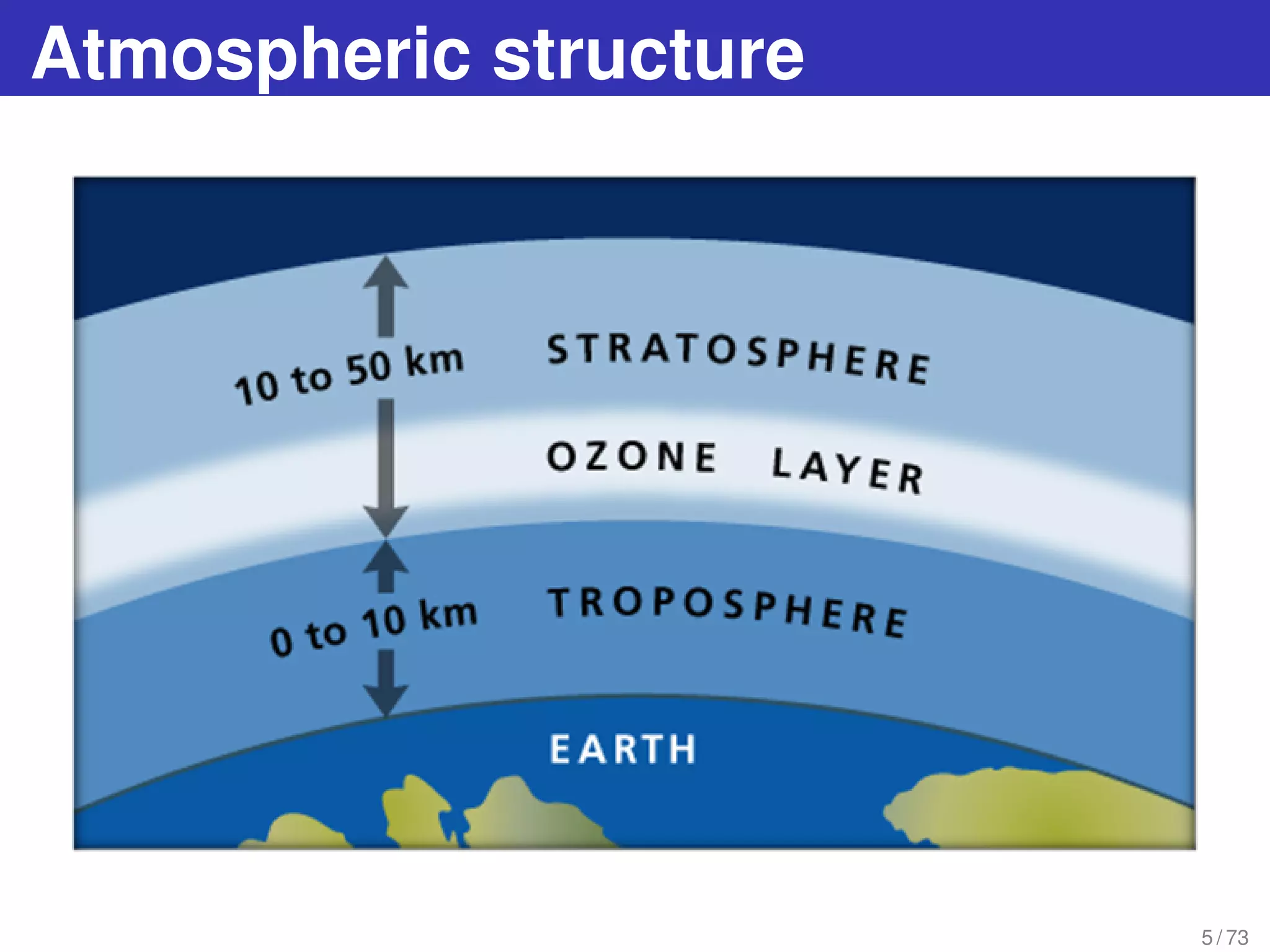
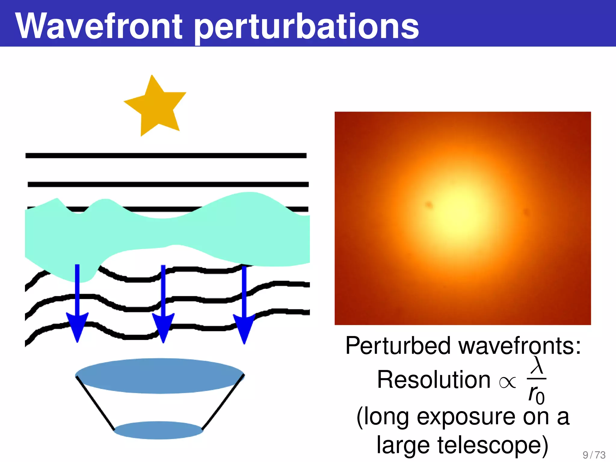
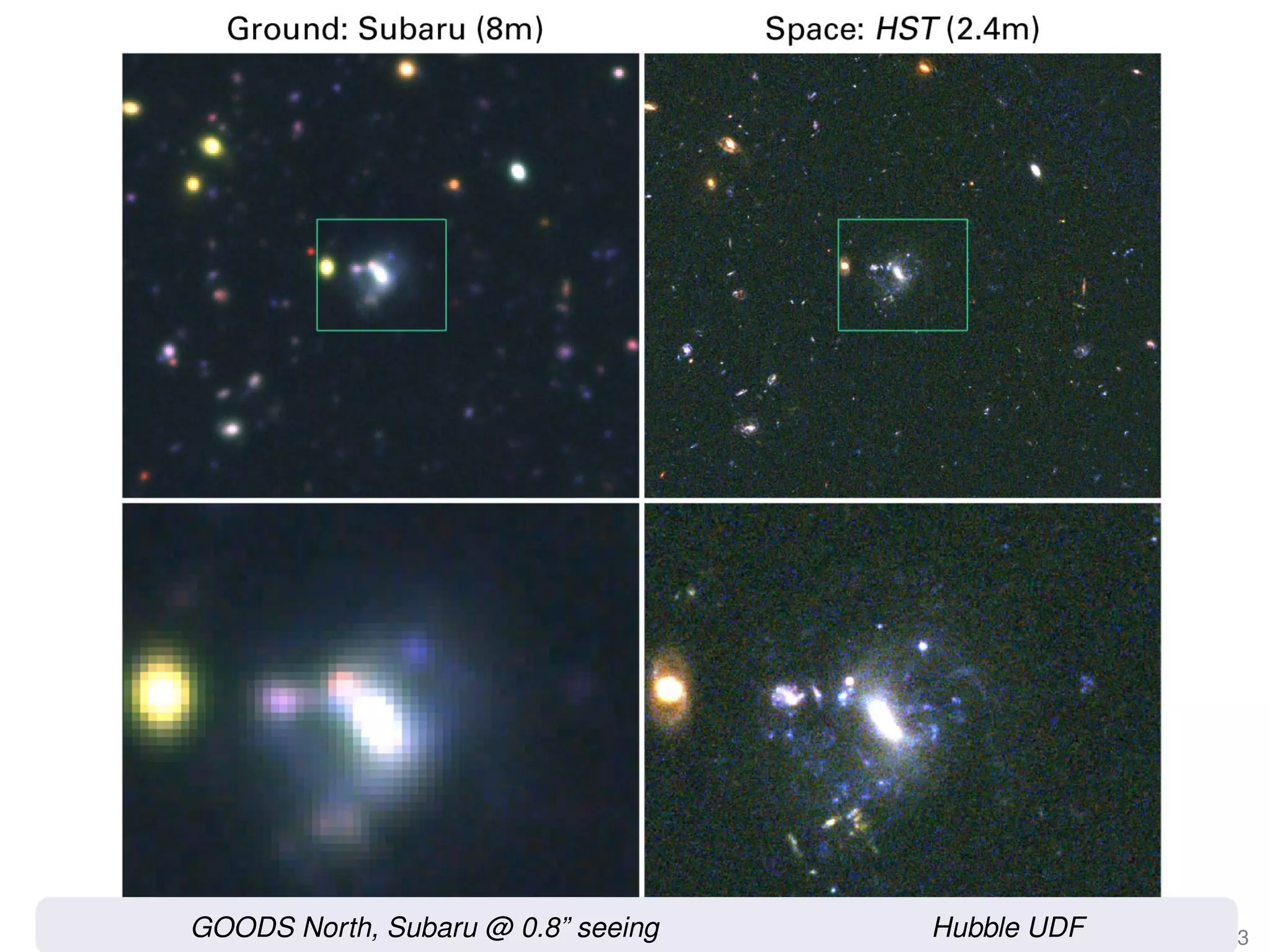
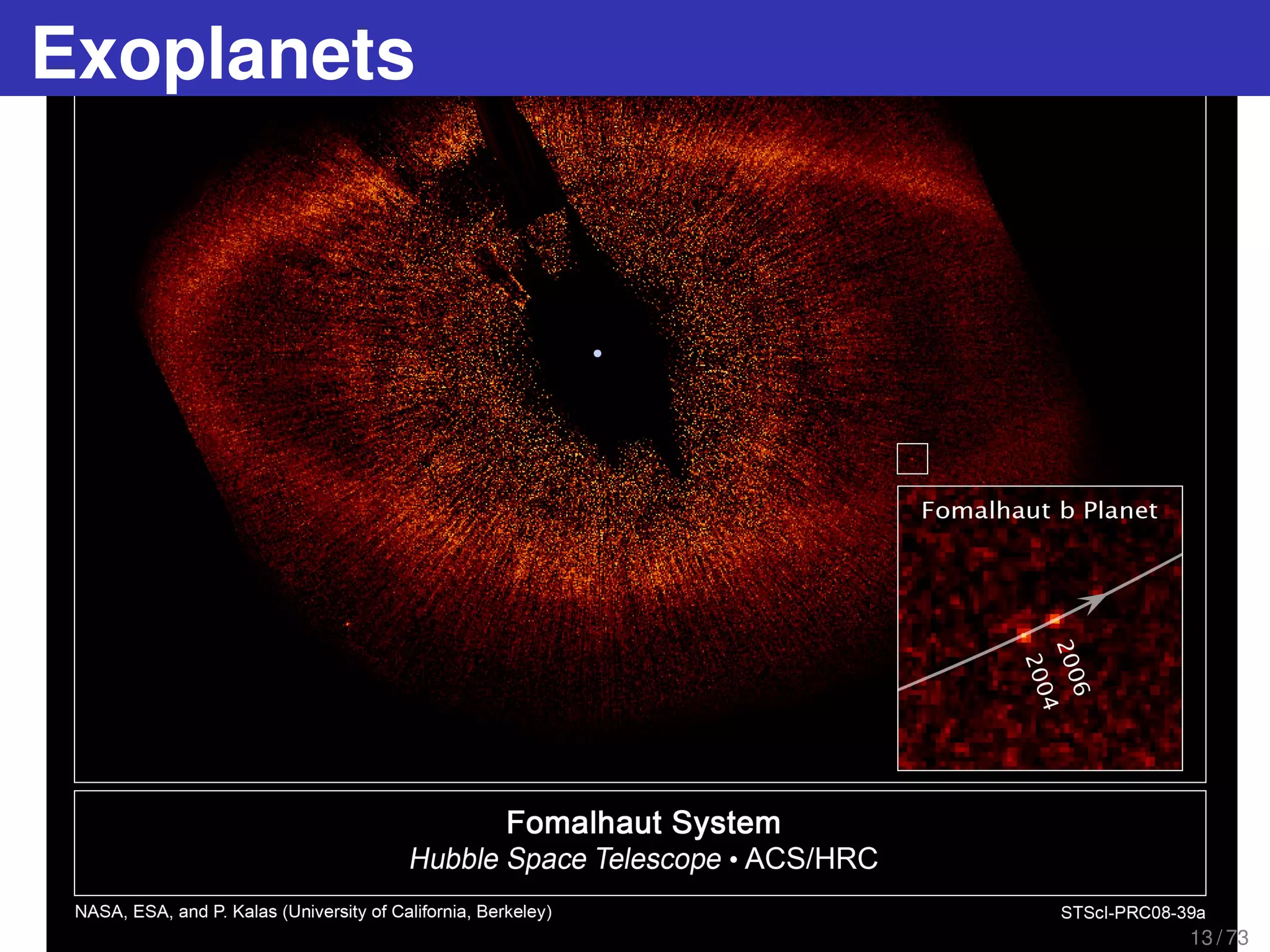
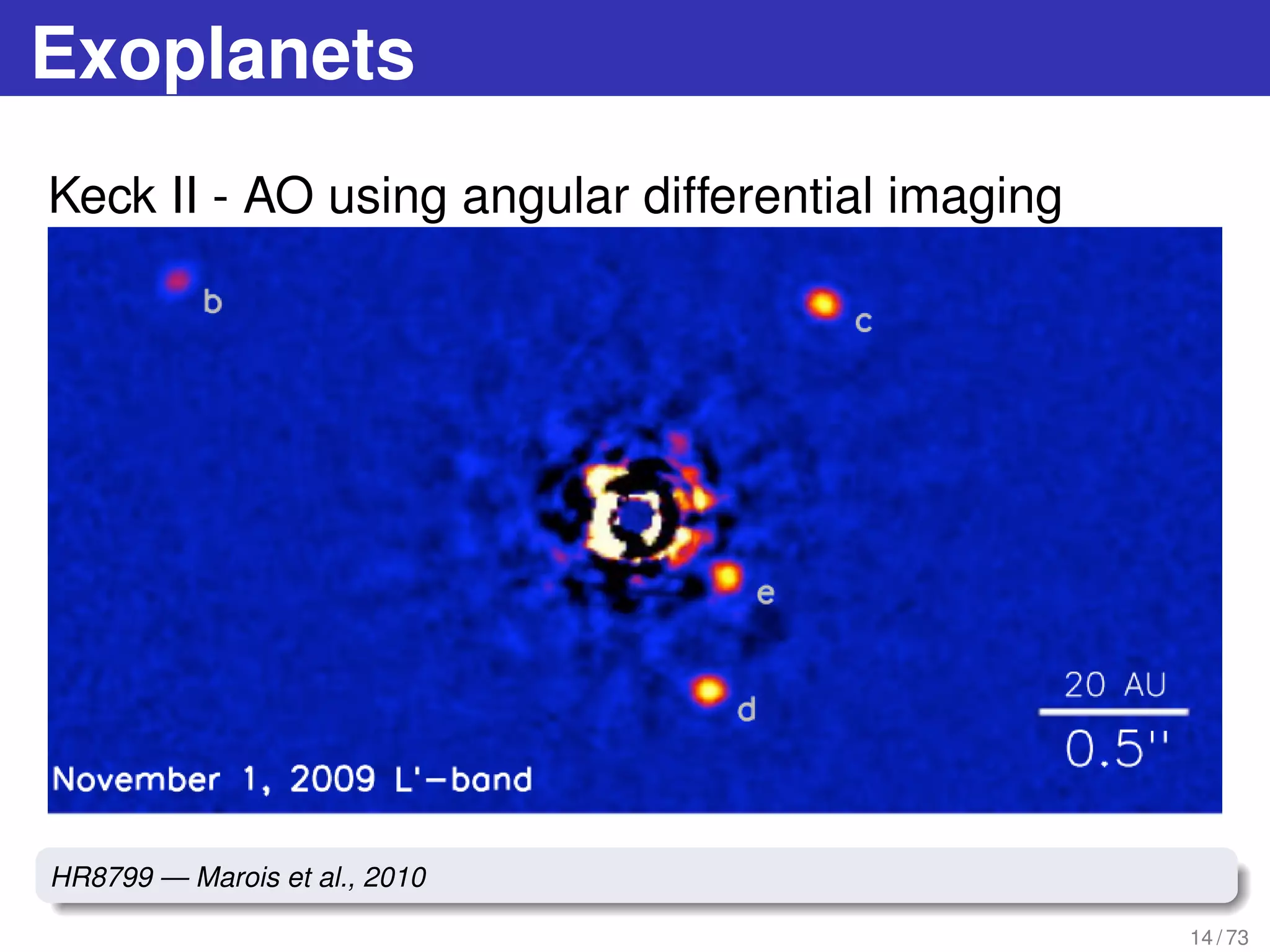
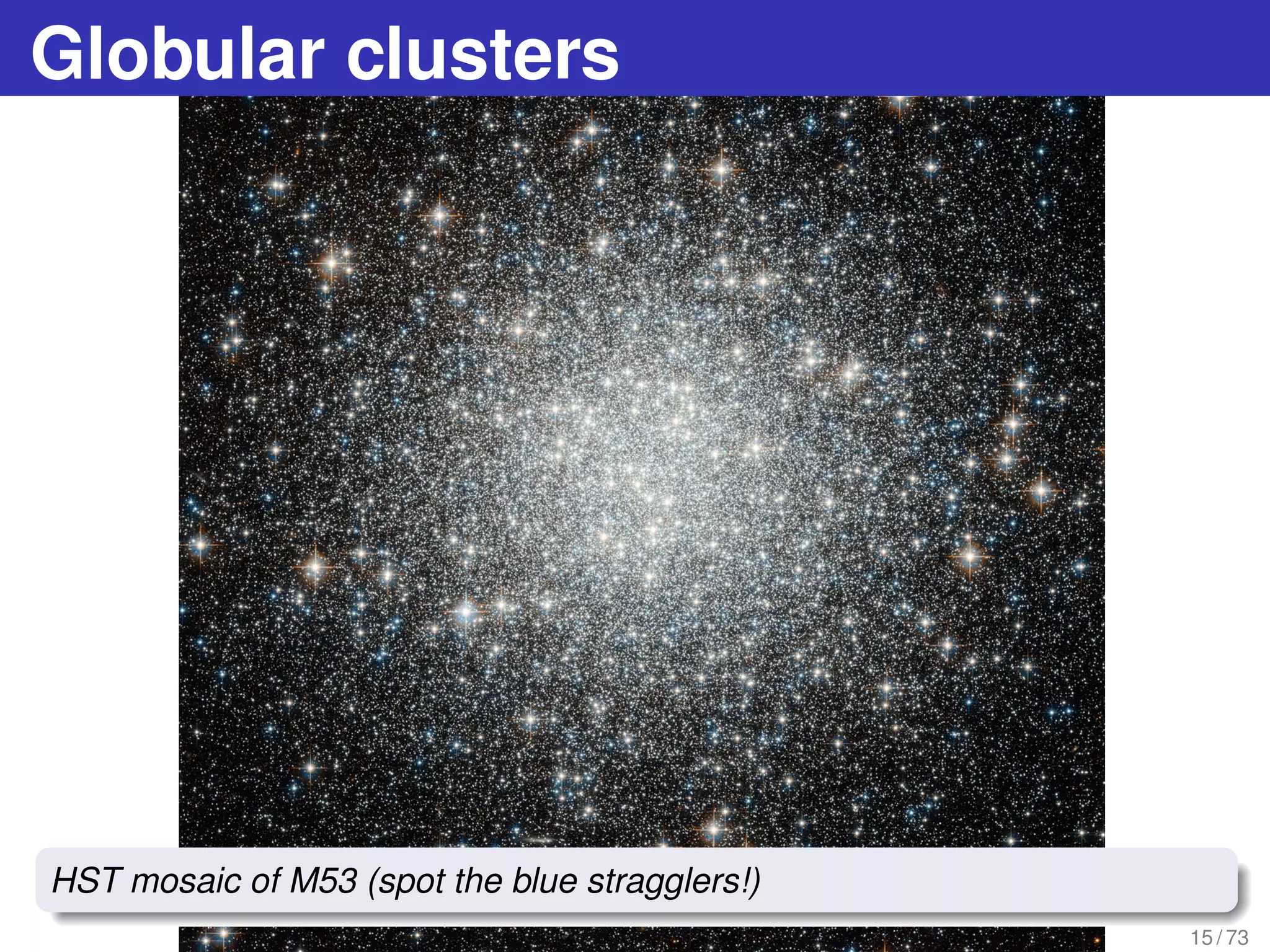
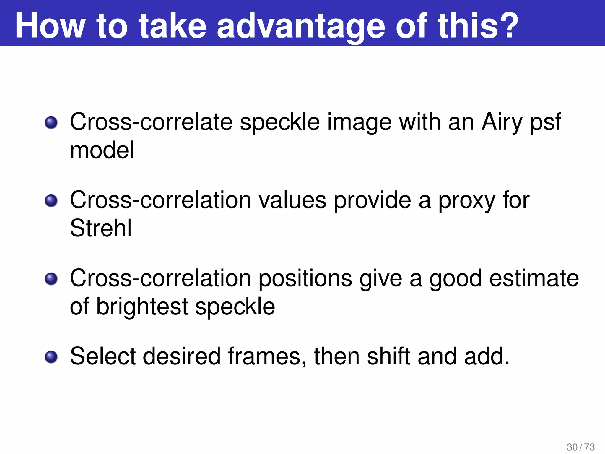
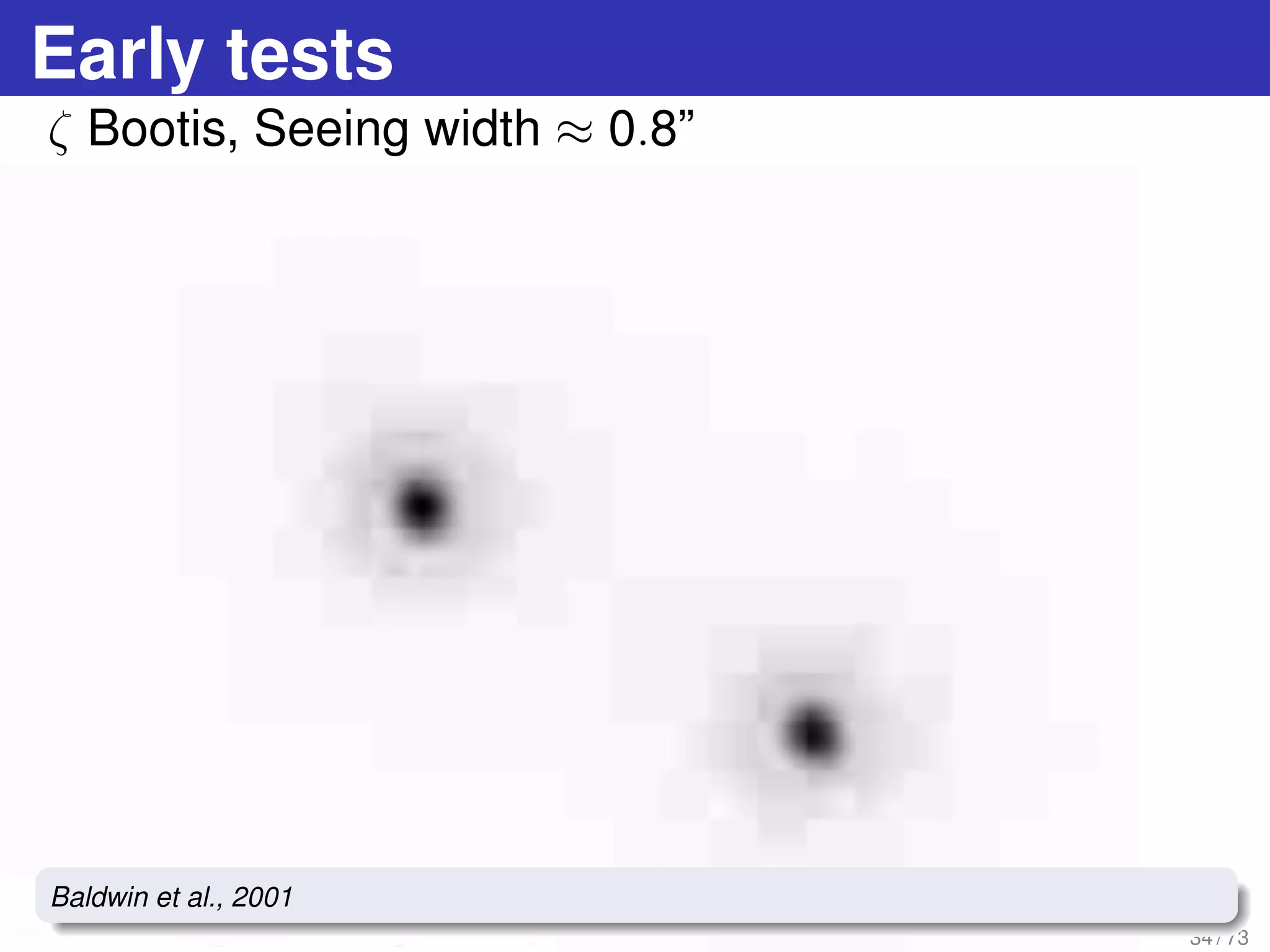
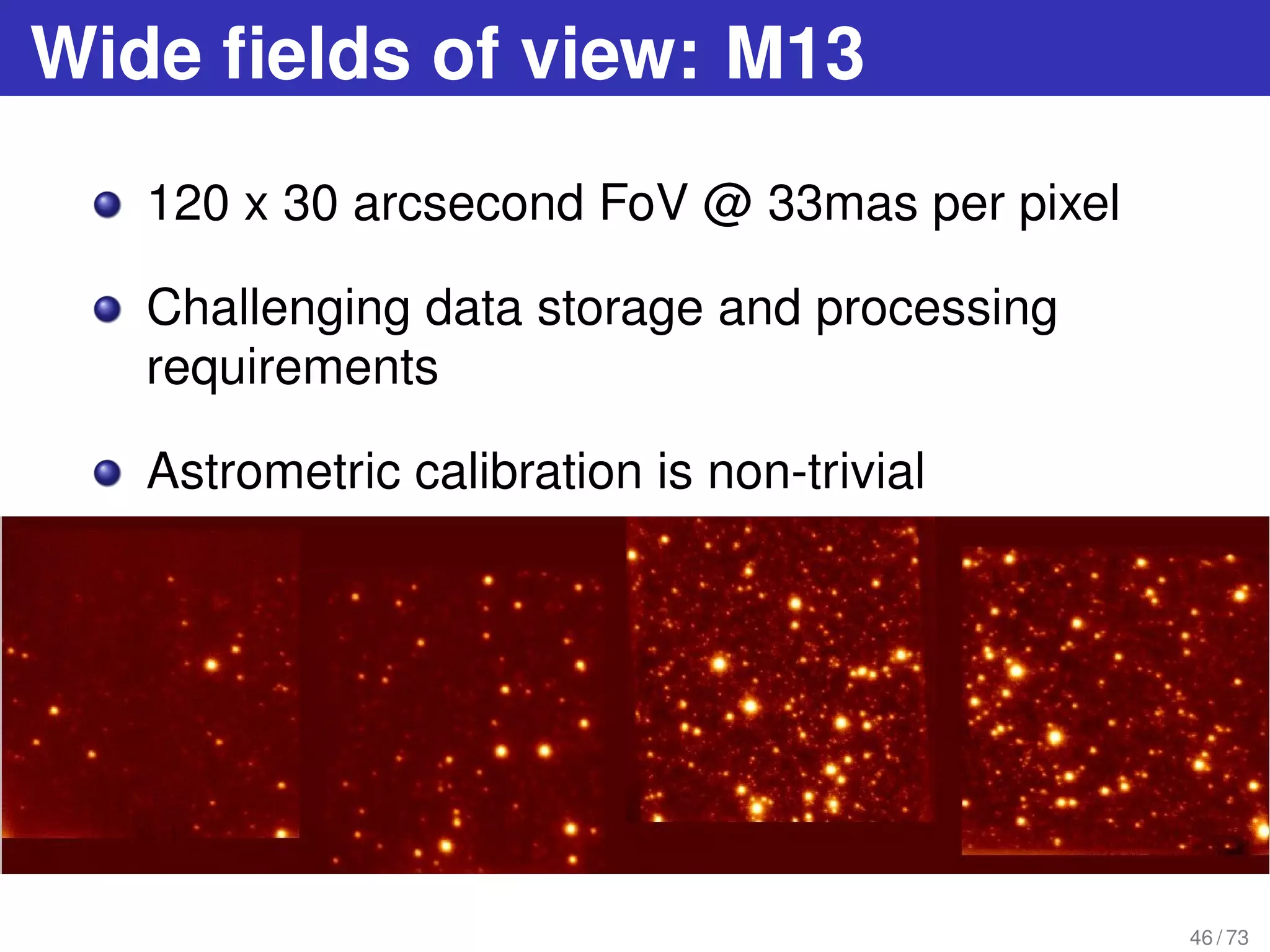
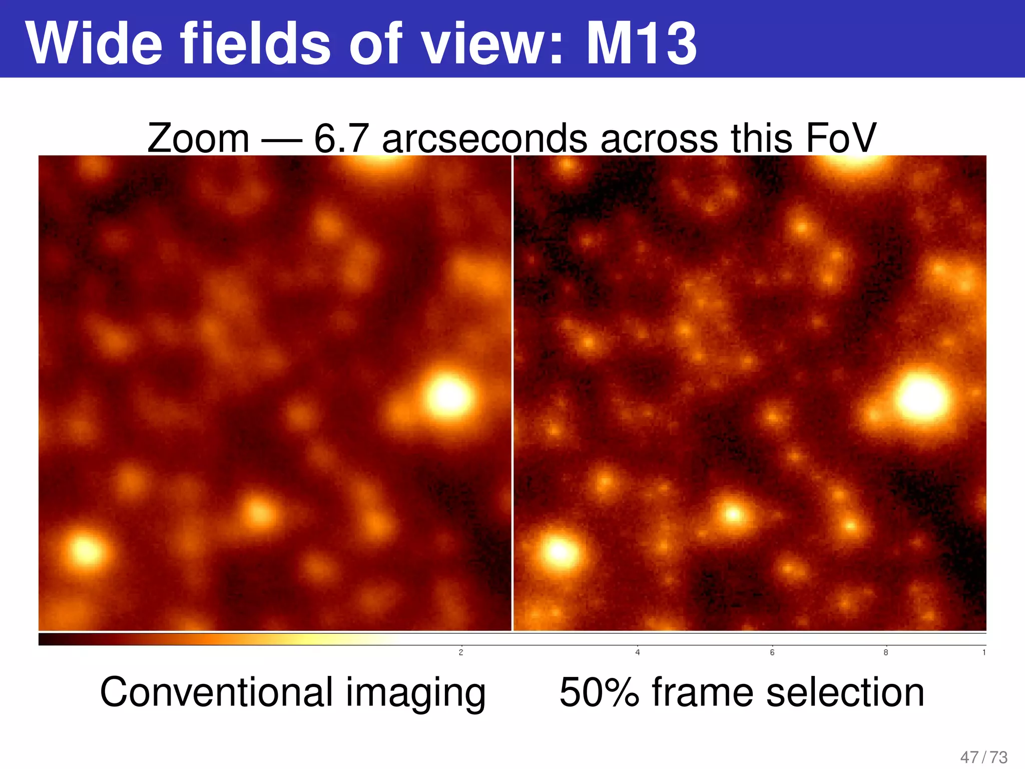
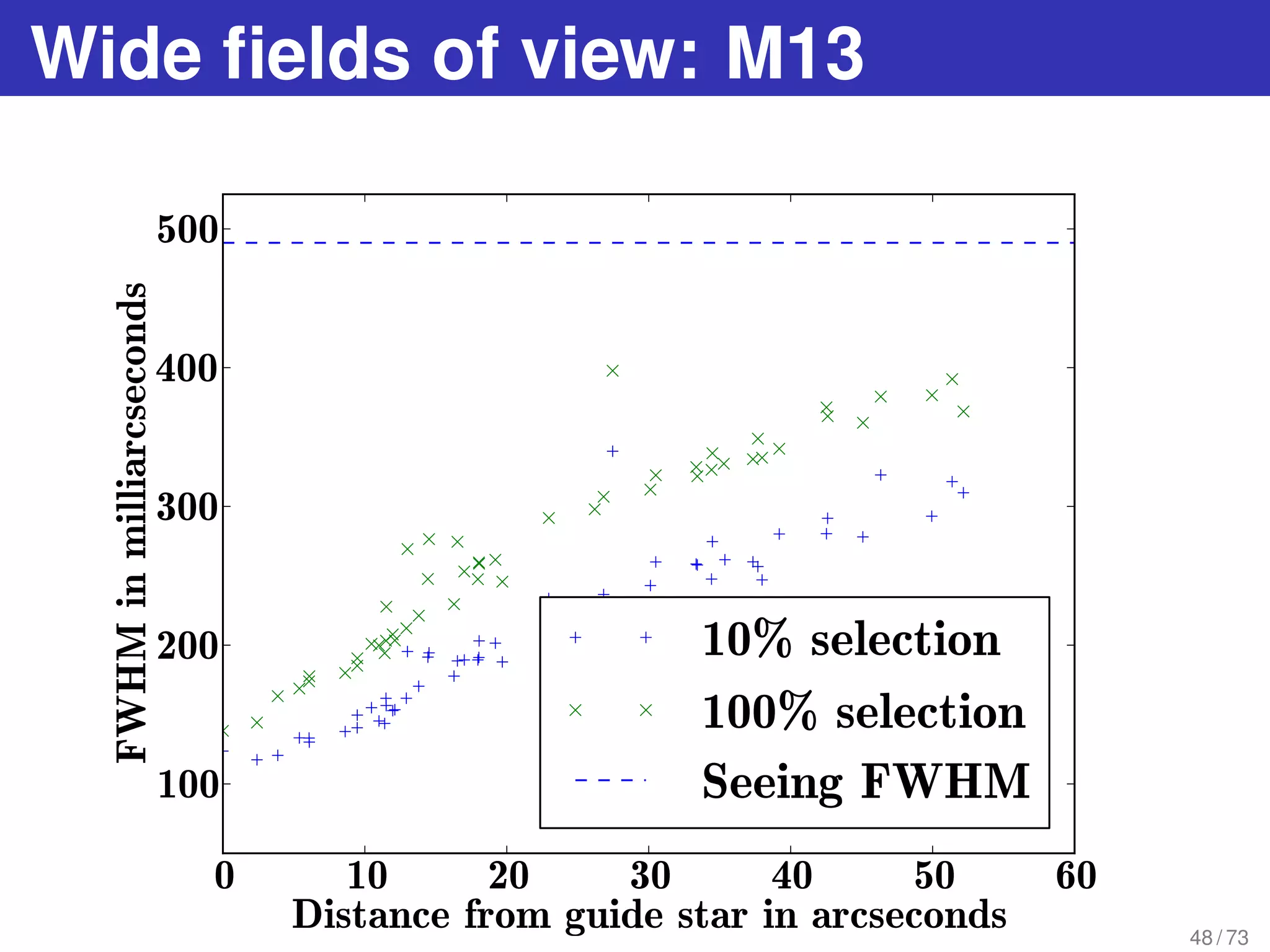
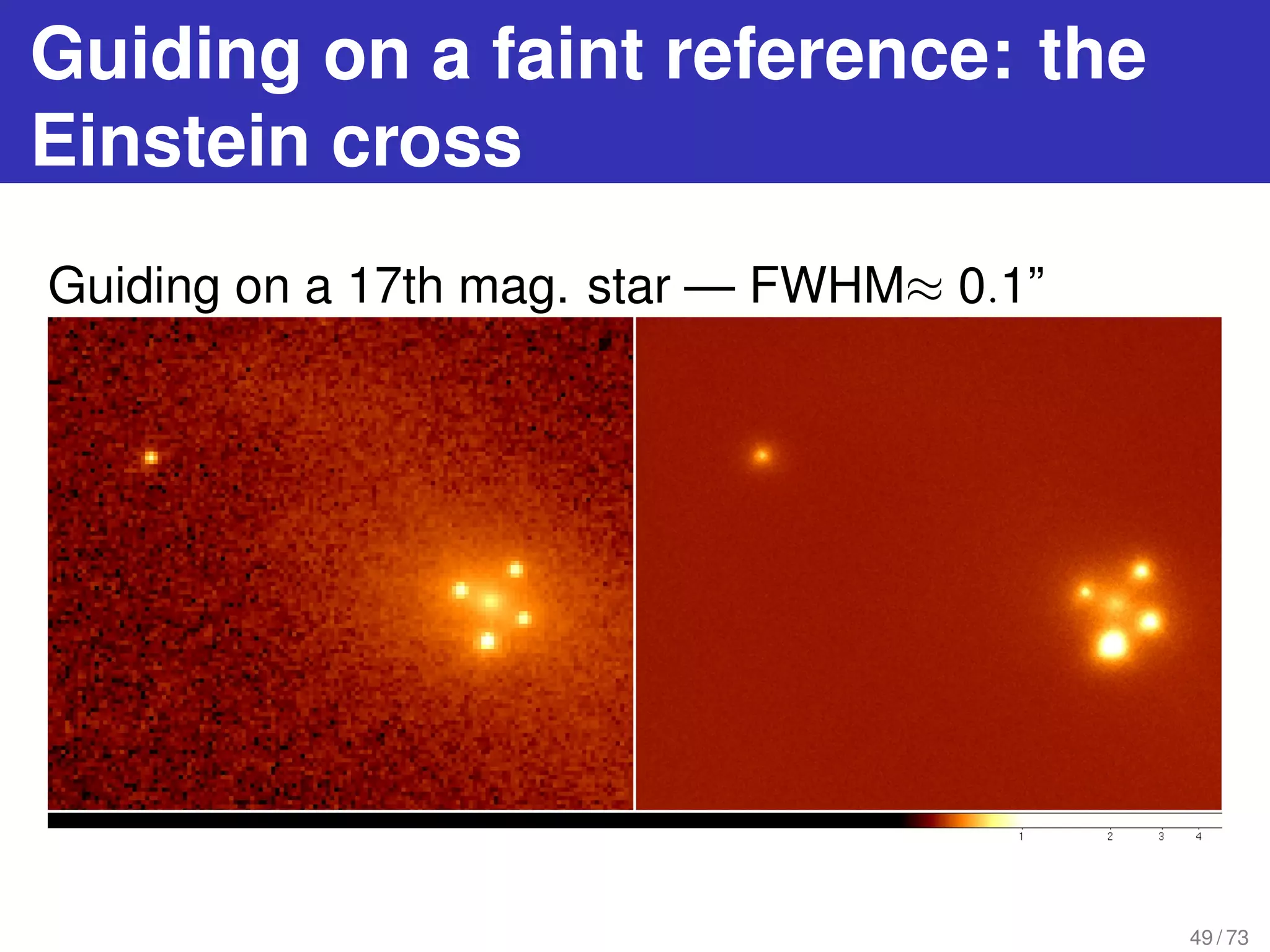
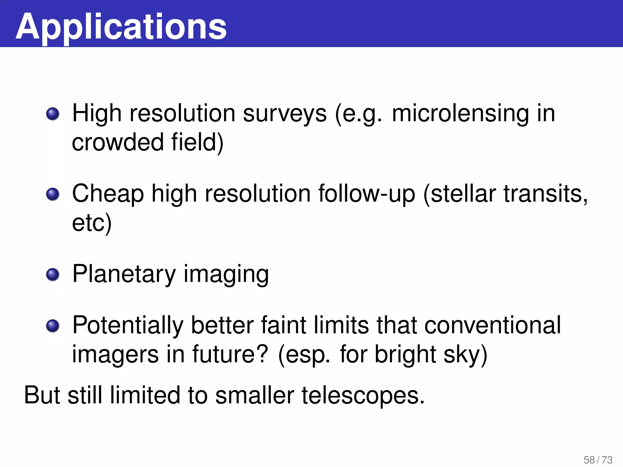
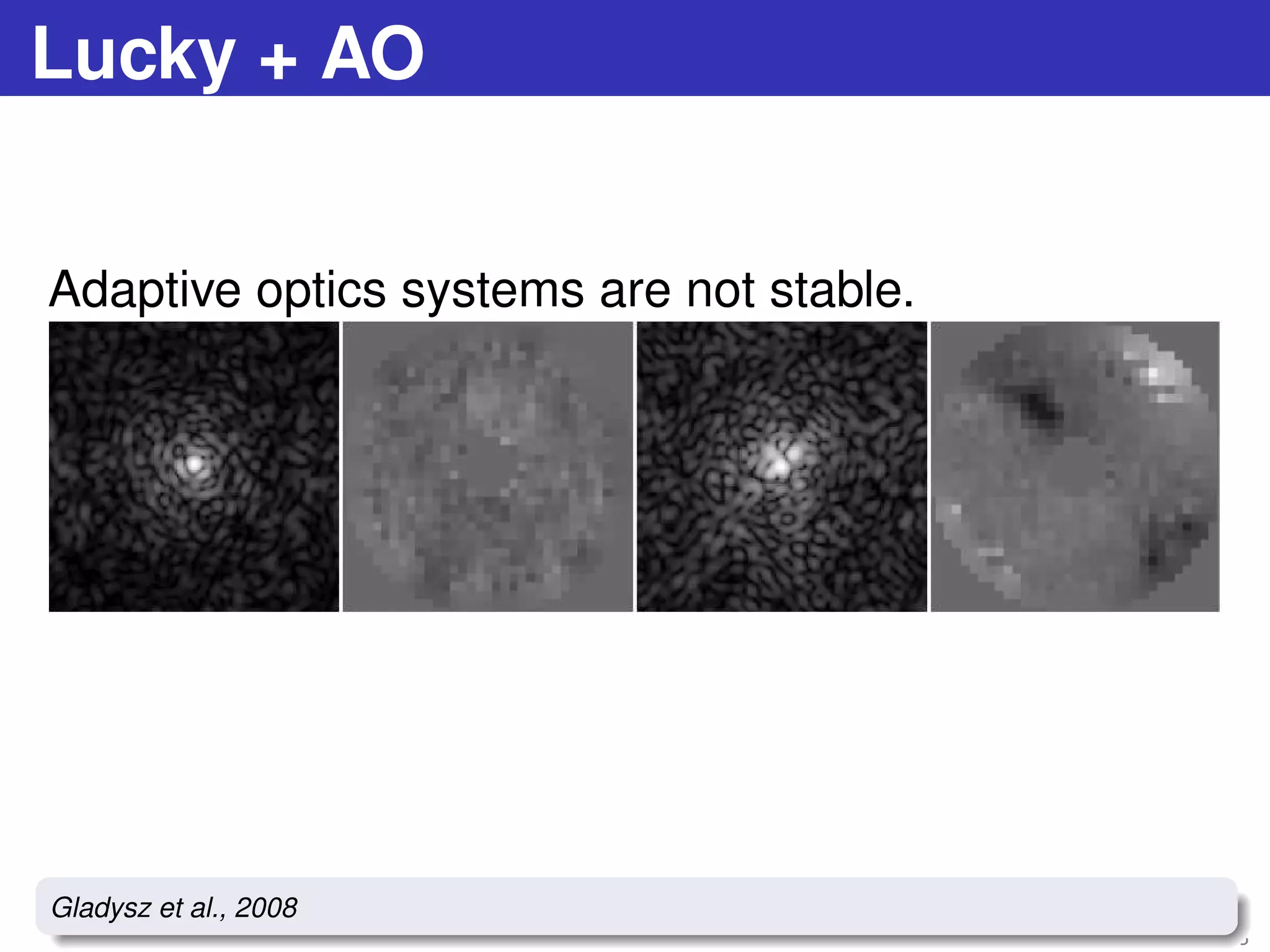
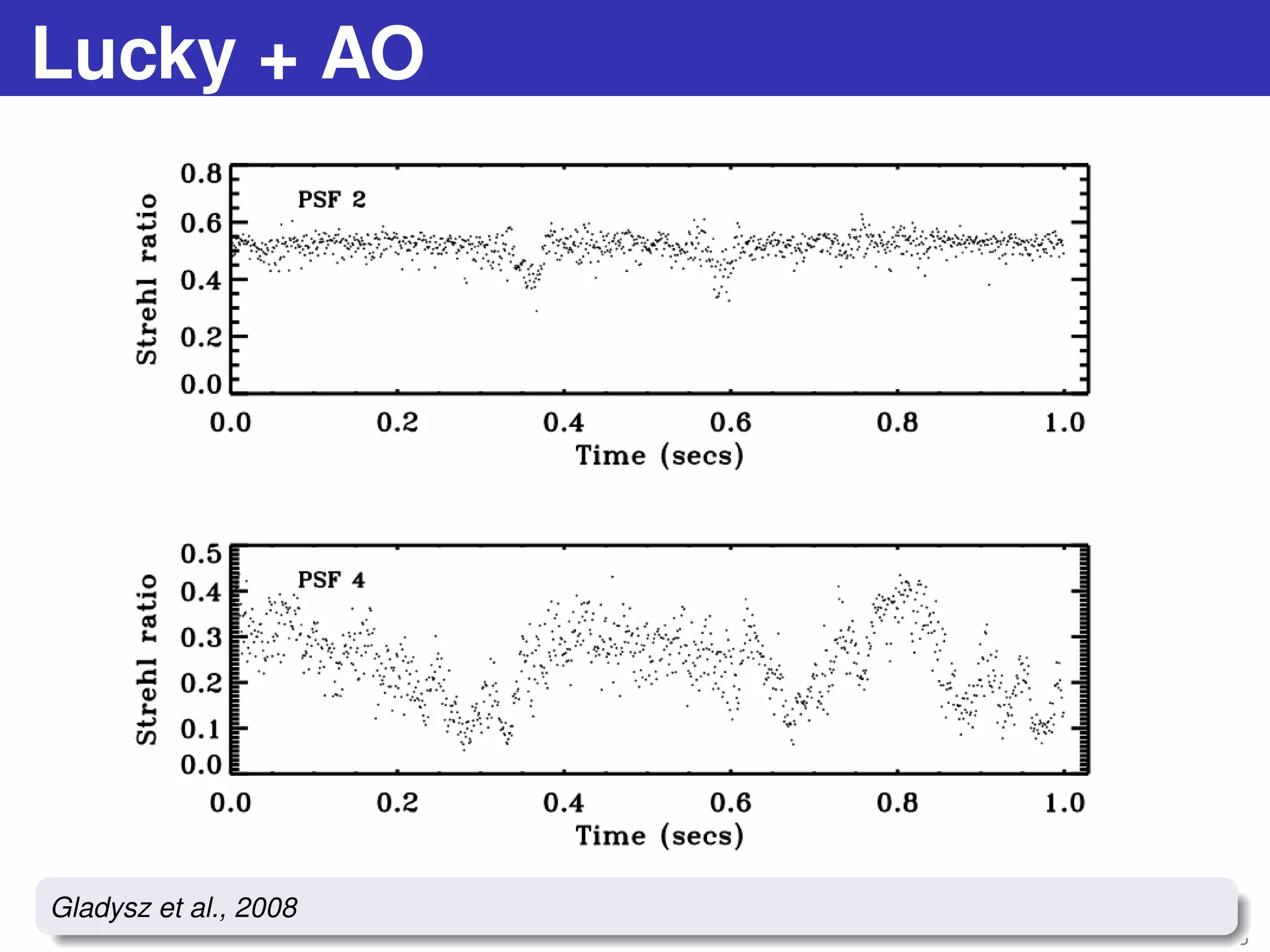
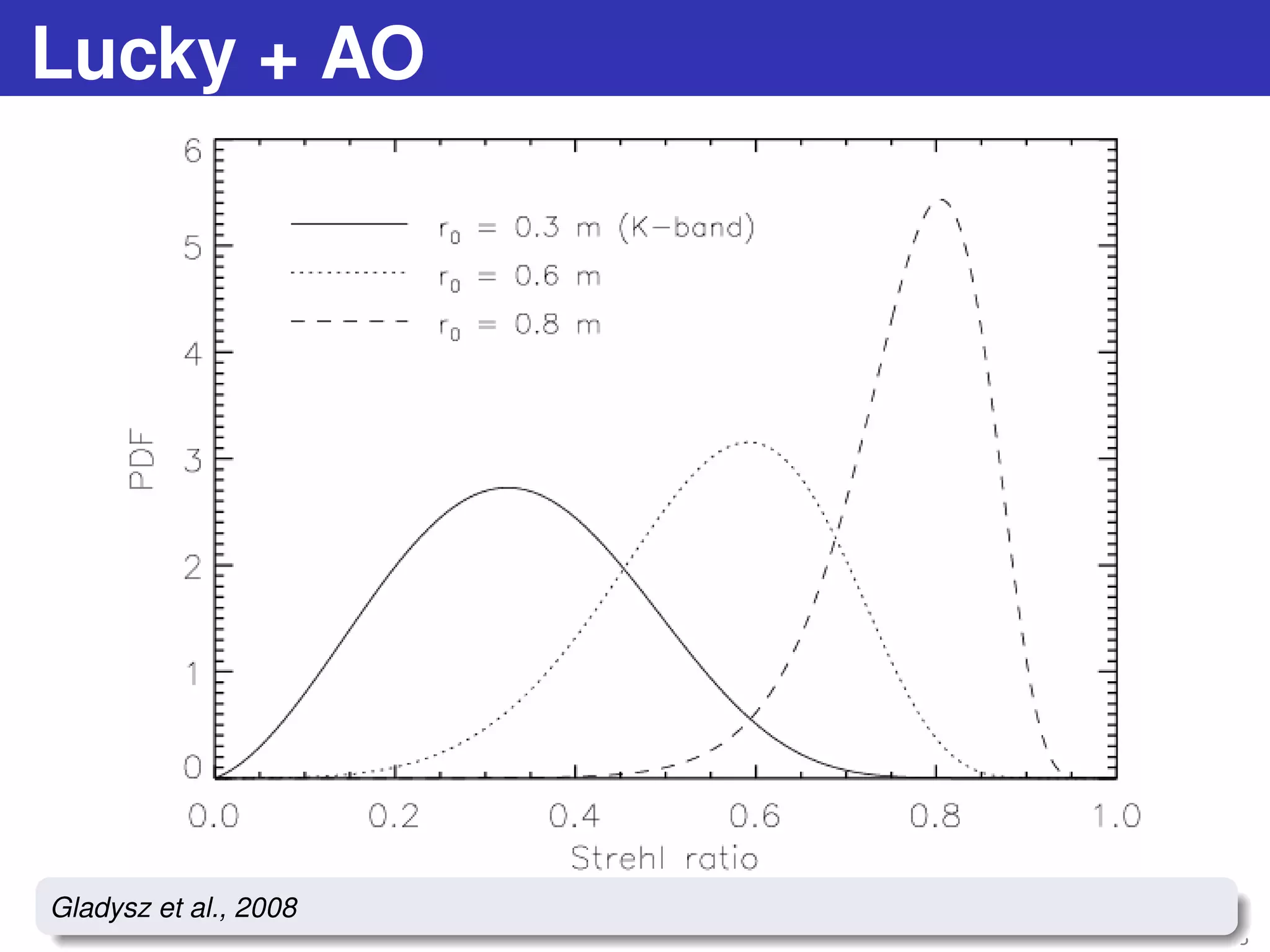
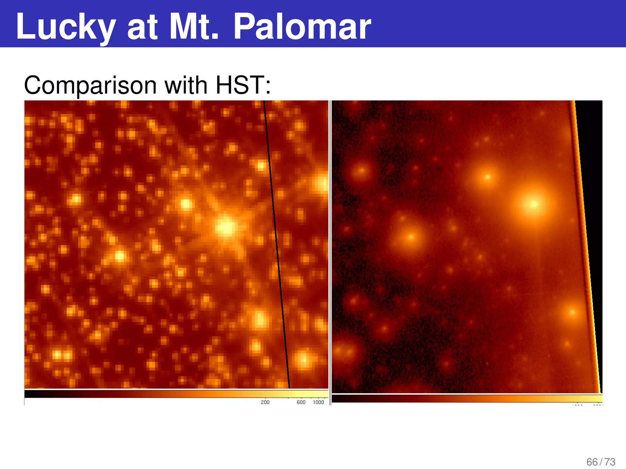
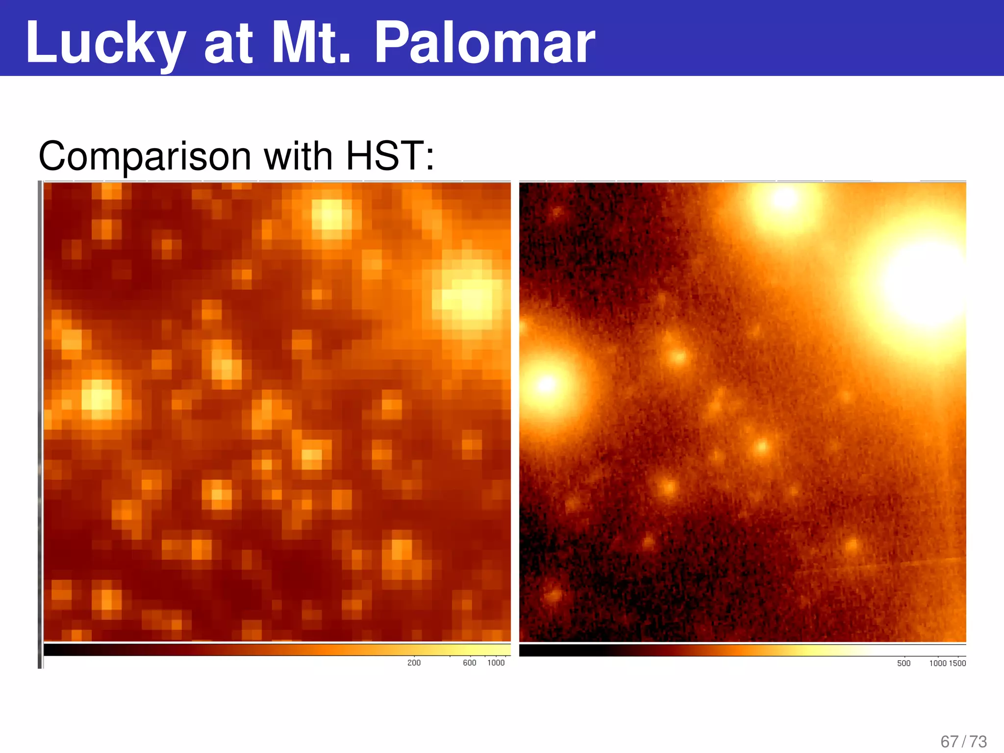
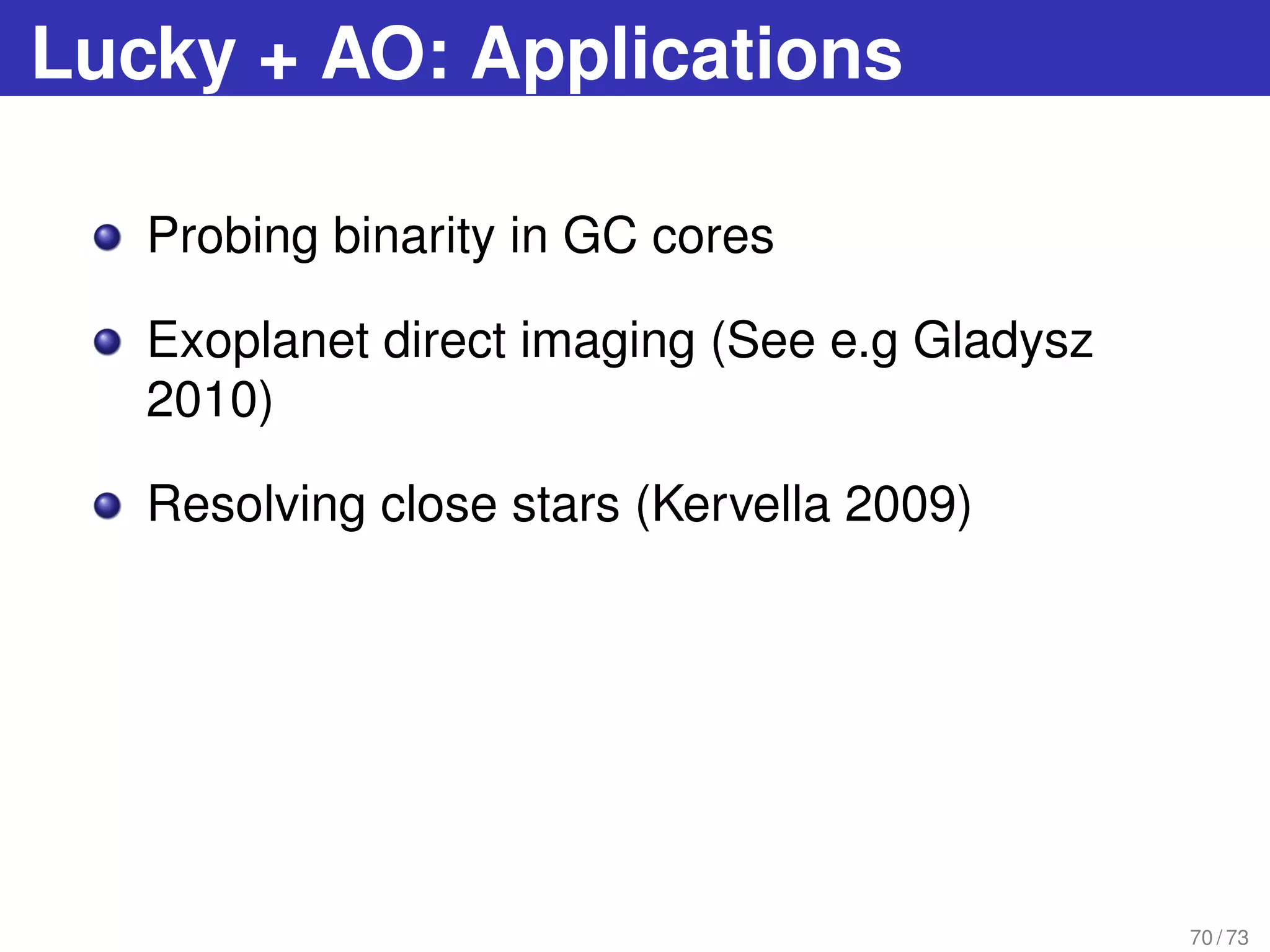
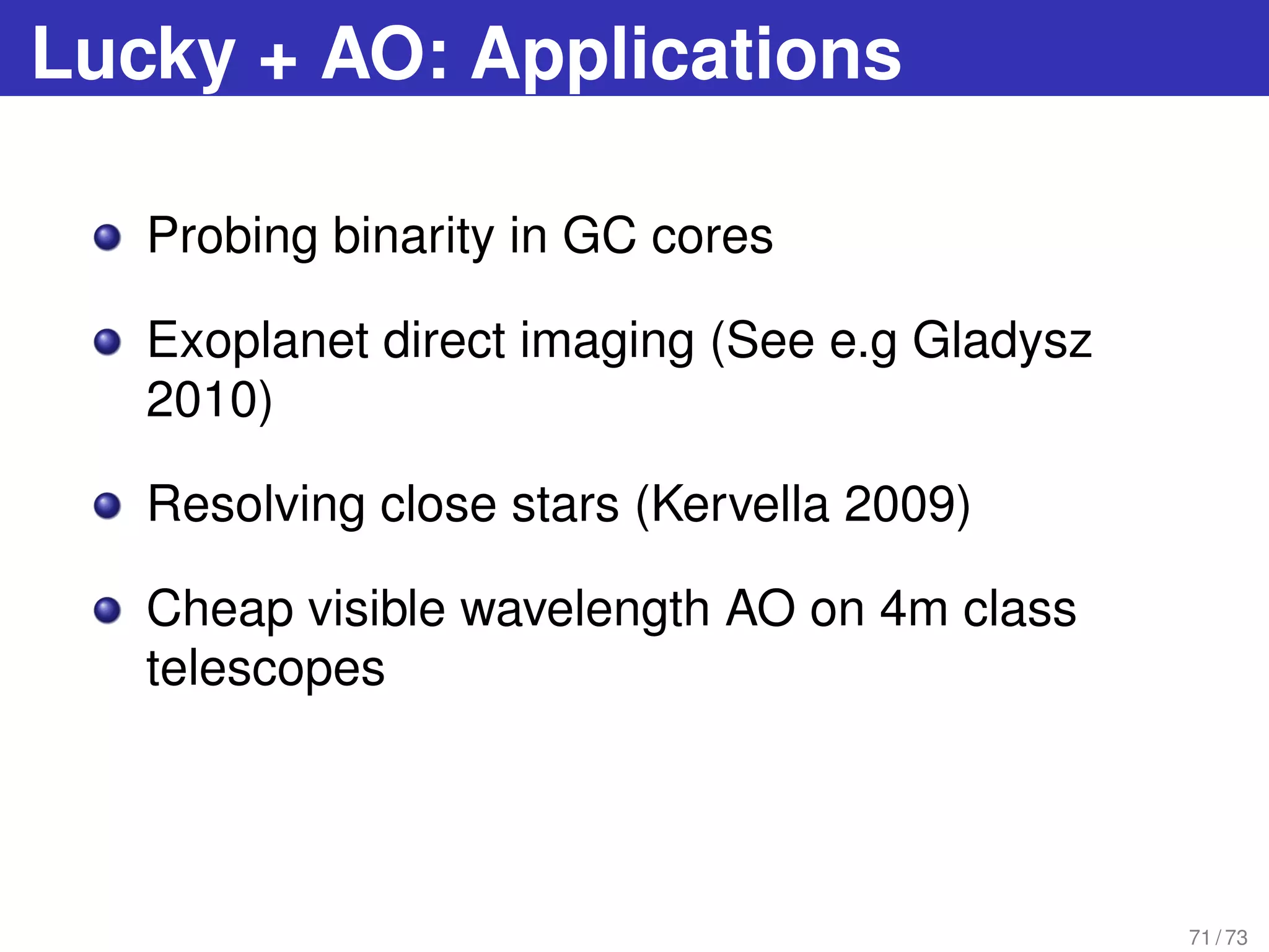
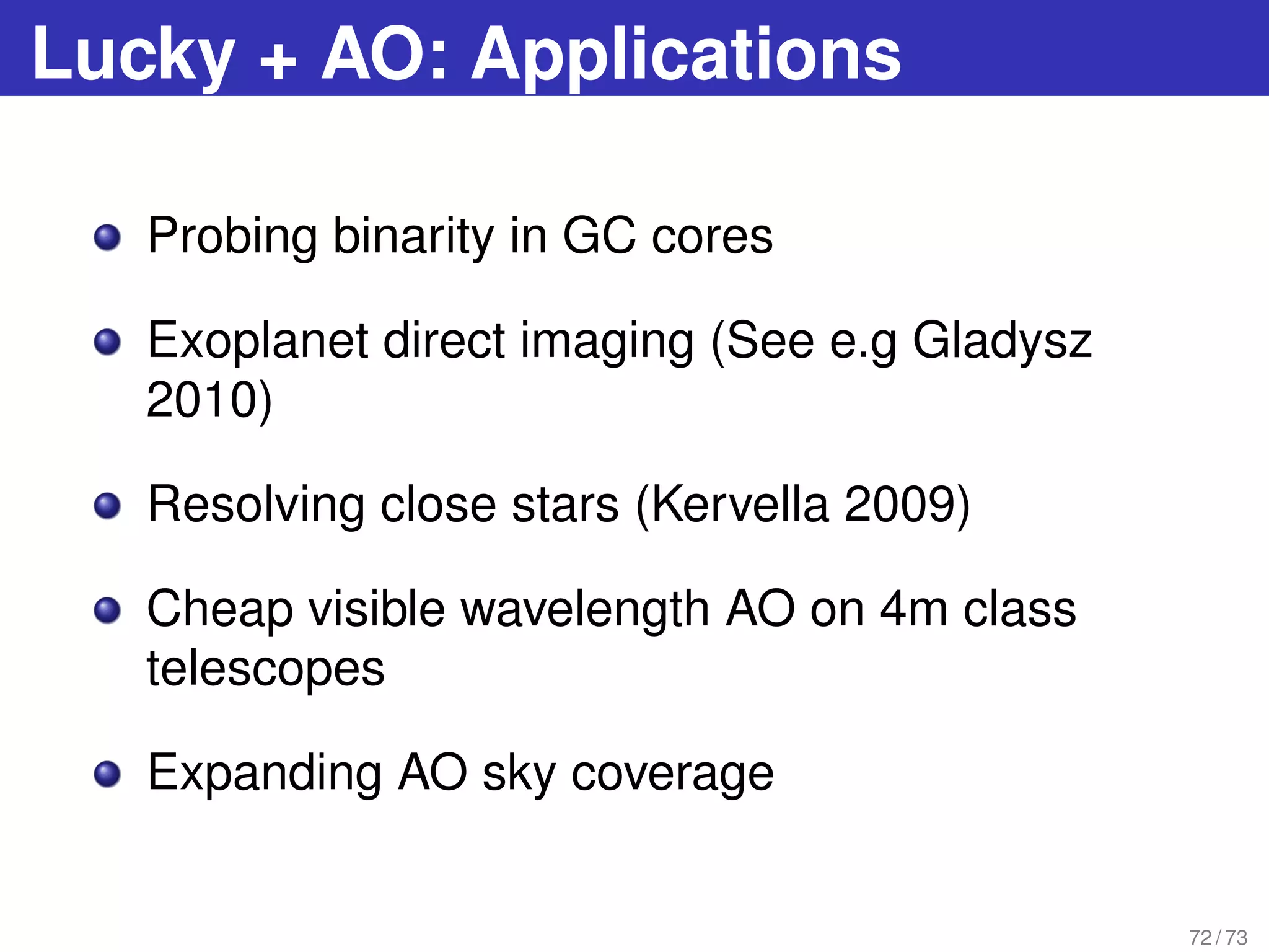
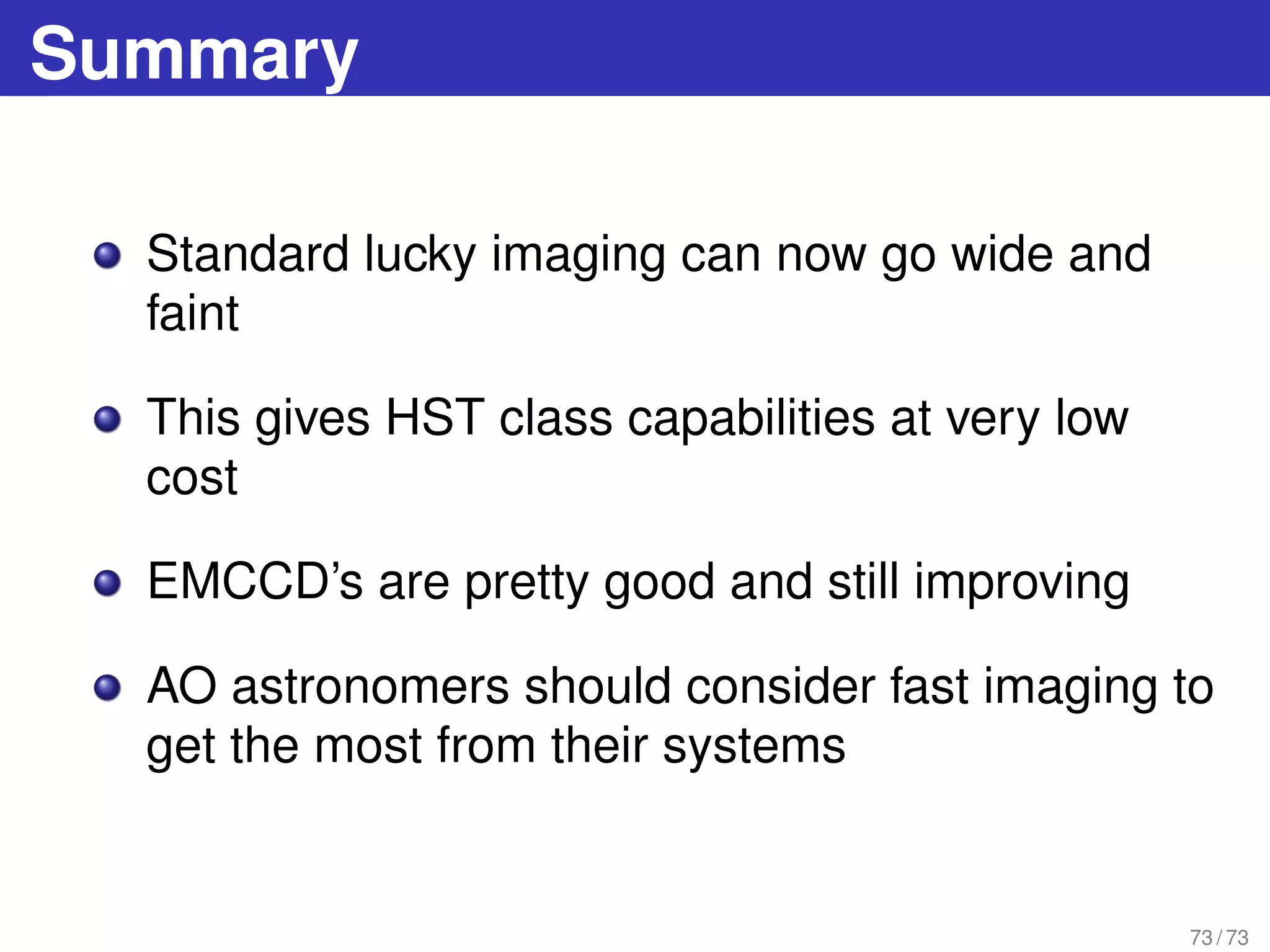
1. Lucky Imaging
Life in the visible after HST
Tim Staley
Southampton Seminar Series
February 2012
WWW: timstaley.co.uk 1 / 73

2. Outline
1 Atmospheric effects
2 High spatial resolution astronomy
3 Adaptive optics
4 Lucky imaging
5 Lucky imaging + AO
2 / 73

3. Outline
1 Atmospheric effects
2 High spatial resolution astronomy
3 Adaptive optics
4 Lucky imaging
5 Lucky imaging + AO
3 / 73

4. Coping with weather
4 / 73

5. Atmospheric structure
5 / 73

6. Boundary layers
6 / 73

7. Kelvin-Helmholtz instability –>
turbulence
7 / 73

8. Wavefront perturbations
Planar wavefronts:
Resolution ∝
λ
D 8 / 73

9. Wavefront perturbations
Perturbed wavefronts:
Resolution ∝
λ
r0
(long exposure on a
large telescope) 9 / 73

10. 10 / 73GOODS North, Subaru @ 0.8” seeing Hubble UDF

11. Outline
1 Atmospheric effects
2 High spatial resolution astronomy
3 Adaptive optics
4 Lucky imaging
5 Lucky imaging + AO
11 / 73

12. Why bother?
12 / 73

13. Exoplanets
13 / 73

14. Exoplanets
Keck II - AO using angular differential imaging
14 / 73
HR8799 — Marois et al., 2010

15. Globular clusters
15 / 73
HST mosaic of M53 (spot the blue stragglers!)

16. 16 / 73

17. The cost of space astronomy
HST:
≈ $2 billion at launch
(1990)
$9.6 billion lifetime cost,
including servicing
missions
17 / 73
Image: ESA
Source: NY Times: “Refurbishments Complete, Astronauts Let Go of Hubble”

18. Ground based astronomy
VLT:
$330 Me to build
$16.9 Me annual
running costs
‘Expensive’ is relative
18 / 73
Image: ESA
Source: www.eso.org

19. Outline
1 Atmospheric effects
2 High spatial resolution astronomy
3 Adaptive optics
4 Lucky imaging
5 Lucky imaging + AO
19 / 73

20. AO: The basic idea
20 / 73

21. Guide stars and sky coverage
Isoplanatic patch = area
for which perturbations
roughly the same
Require rmag ≤ 10 star
within 5” – 40”, depending
on observation
wavelength and
atmospheric conditions
21 / 73
See e.g. Racine, 2006

22. Laser guide stars
22 / 73
Image: G. Hudepohl / ESO

23. Laser guide stars
23 / 73
Image: R. Tyson - An introduction to AO (2000)

24. Laser guide stars
Still require a tip-tilt NGS of
rmag ≤ 14 within ≈ 40” of
science target.
Good quality sky coverage
≈ 10% at 30◦
galactic latitude.
(Strehl ≥ 0.3, J band)
24 / 73
Davies et al., 2008
Ellerbroek and Tyler, 1998

25. (Strehl?)
The ratio of peak intensity compared to a perfect
telescope (0 to 1)
HST Strehl near 1, but suffers pixellation effects.
AO Strehl usually varies from around 0.2 – 0.6
Seeing “Strehl” depends on the telescope, but is
typically ≈ 0.01 on medium size telescopes in
the visible.
25 / 73

26. Outline
1 Atmospheric effects
2 High spatial resolution astronomy
3 Adaptive optics
4 Lucky imaging
5 Lucky imaging + AO
26 / 73

27. Seeing isn’t stable
How often will we get a ‘good’ frame?
27 / 73

28. Fried’s probabilities
Probability of a lucky exposure
(near diffraction limited):
P ≈ 5.6 exp − 0.1557(D/r0)2
28 / 73
Fried, 1978

29. Fried’s probabilities
D/r0 Probability
2 0.986 ± 0.006
3 0.765 ± 0.005
4 0.334 ± 0.014
5 (9.38 ± 0.33) × 10−2
6 (1.915 ± 0.084) × 10−2
7 (2.87 ± 0.57) × 10−3
10 (1.07 ± 0.48) × 10−6
15 (3.40 ± 0.59) × 10−15
29 / 73
Fried, 1978

30. How to take advantage of this?
Cross-correlate speckle image with an Airy psf
model
Cross-correlation values provide a proxy for
Strehl
Cross-correlation positions give a good estimate
of brightest speckle
Select desired frames, then shift and add.
30 / 73

31. Early tests
31 / 73

32. Early tests
2.5m Nordic Optical Telescope
512 sq. pixel detector
185Hz frame rate
810nm observing wavelength
Faint limit at 6th magnitude
32 / 73

33. Early tests
Seeing width ≈ 0.4”
33 / 73
Baldwin et al., 2001

34. Early tests
ζ Bootis, Seeing width ≈ 0.8”
34 / 73
Baldwin et al., 2001

35. Fast imaging with EMCCD’s
35 / 73
Cost: Around £15K

36. Fast imaging with EMCCD’s
Conventional CCD:
SNR= M√
M+σ2
N
EMCCD:
SNR= M√
2M+(σN /gA)2
36 / 73

37. Fast imaging with EMCCD’s
Calibration:
37 / 73

38. Fast imaging with EMCCD’s
Calibration:
38 / 73

39. Fast imaging with EMCCD’s
Calibration:
39 / 73

40. Fast imaging with EMCCD’s
Limited pixel size, 1K2
Can only get 30 sq. arcseconds Nyquist
sampled on 2.5m telescope.
Readout electronics are a bottleneck on the
frame rate
40 / 73

41. 2009 — LuckyCam goes wide field
41 / 73

42. 2009 — LuckyCam goes wide field
42 / 73

43. 2009 — LuckyCam goes wide field
43 / 73

44. 2009 — LuckyCam goes wide field
44 / 73

45. 2009 — LuckyCam goes wide field
45 / 73

46. Wide fields of view: M13
120 x 30 arcsecond FoV @ 33mas per pixel
Challenging data storage and processing
requirements
Astrometric calibration is non-trivial
46 / 73

47. Wide fields of view: M13
Zoom — 6.7 arcseconds across this FoV
Conventional imaging 50% frame selection
47 / 73

48. Wide fields of view: M13
0 10 20 30 40 50 60
Distance from guide star in arcseconds
100
200
300
400
500
FWHMinmilliarcseconds
10% selection
100% selection
Seeing FWHM
48 / 73

49. Guiding on a faint reference: the
Einstein cross
Guiding on a 17th mag. star — FWHM≈ 0.1”
49 / 73

50. Science at the faint limit:
thresholding
Read out noise still 0.1 electrons.
Faint limit around 23rd magnitude on a 2.5m
telescope (good seeing)
Thresholding eliminates read noise
But for now we are limited by CIC
50 / 73

51. Science at the faint limit:
thresholding
51 / 73

52. Science at the faint limit:
thresholding
52 / 73

53. Applications
Stellar binarity surveys
53 / 73

54. Applications
High resolution surveys (e.g. microlensing in
crowded field)
54 / 73

55. Applications
High resolution surveys (e.g. microlensing in
crowded field)
Cheap high resolution follow-up (stellar transits,
etc)
55 / 73

56. Applications
High resolution surveys (e.g. microlensing in
crowded field)
Cheap high resolution follow-up (stellar transits,
etc)
Planetary imaging
56 / 73

57. Applications
High resolution surveys (e.g. microlensing in
crowded field)
Cheap high resolution follow-up (stellar transits,
etc)
Planetary imaging
Potentially better faint limits that conventional
imagers in future? (esp. for bright sky)
57 / 73

58. Applications
High resolution surveys (e.g. microlensing in
crowded field)
Cheap high resolution follow-up (stellar transits,
etc)
Planetary imaging
Potentially better faint limits that conventional
imagers in future? (esp. for bright sky)
But still limited to smaller telescopes.
58 / 73

59. Outline
1 Atmospheric effects
2 High spatial resolution astronomy
3 Adaptive optics
4 Lucky imaging
5 Lucky imaging + AO
59 / 73

60. Lucky + AO
Adaptive optics systems are not stable.
60 / 73
Gladysz et al., 2008

61. Lucky + AO
61 / 73
Gladysz et al., 2008

62. Lucky + AO
62 / 73
Gladysz et al., 2008

63. Lucky at Mt. Palomar
63 / 73
Law et al., 2009

64. Lucky at Mt. Palomar
5m Palomar “200 inch” Hale telescope
512 sq. pixel EMCCD detector
First generation AO system (since upgraded)
64 / 73
Law et al., 2009

65. Lucky at Mt. Palomar
Field of view:
65 / 73

66. Lucky at Mt. Palomar
Comparison with HST:
66 / 73

67. Lucky at Mt. Palomar
Comparison with HST:
67 / 73

68. Lucky + AO: Applications
Probing binarity in GC cores
68 / 73

69. Lucky + AO: Applications
Probing binarity in GC cores
Exoplanet direct imaging (See e.g Gladysz
2010)
69 / 73

70. Lucky + AO: Applications
Probing binarity in GC cores
Exoplanet direct imaging (See e.g Gladysz
2010)
Resolving close stars (Kervella 2009)
70 / 73

71. Lucky + AO: Applications
Probing binarity in GC cores
Exoplanet direct imaging (See e.g Gladysz
2010)
Resolving close stars (Kervella 2009)
Cheap visible wavelength AO on 4m class
telescopes
71 / 73

72. Lucky + AO: Applications
Probing binarity in GC cores
Exoplanet direct imaging (See e.g Gladysz
2010)
Resolving close stars (Kervella 2009)
Cheap visible wavelength AO on 4m class
telescopes
Expanding AO sky coverage
72 / 73

73. Summary
Standard lucky imaging can now go wide and
faint
This gives HST class capabilities at very low
cost
EMCCD’s are pretty good and still improving
AO astronomers should consider fast imaging to
get the most from their systems
73 / 73