1) The document analyzes the correlation function of the 6dF Galaxy Survey (6dFGS) and detects a Baryon Acoustic Oscillation (BAO) signal. 2) This BAO detection allows constraining the distance-redshift relation at an effective redshift of zeff = 0.106, achieving a distance measure of DV(zeff) = 456 ± 27 Mpc. 3) The low effective redshift of 6dFGS makes it competitive with Cepheids and low-z supernovae in constraining the Hubble constant, yielding a value of H0 = 67 ± 3.2 km s−1 Mpc−1.

1. Mon. Not. R. Astron. Soc. 000, 000–000 (0000) Printed 20 June 2011 (MN L TEX style file v2.2)
A
The 6dF Galaxy Survey: Baryon Acoustic Oscillations and
the Local Hubble Constant
Florian Beutler1⋆ , Chris Blake2, Matthew Colless3, D. Heath Jones3,
Lister Staveley-Smith1, Lachlan Campbell4, Quentin Parker3,5, Will Saunders3,
arXiv:1106.3366v1 [astro-ph.CO] 16 Jun 2011
Fred Watson3
1 International Centre for Radio Astronomy Research (ICRAR), University of Western Australia, 35 Stirling Highway, Perth WA 6009,
Australia
2 Centre for Astrophysics & Supercomputing, Swinburne University of Technology, P.O. Box 218, Hawthorn, VIC 3122, Australia
3 Australian Astronomical Observatory, PO Box 296, Epping NSW 1710, Australia
4 Western Kentucky University, Bowling Green, USA
5 Macquarie University, Sydney, Australia
20 June 2011
ABSTRACT
We analyse the large-scale correlation function of the 6dF Galaxy Survey (6dFGS)
and detect a Baryon Acoustic Oscillation (BAO) signal. The 6dFGS BAO detection
allows us to constrain the distance-redshift relation at zeff = 0.106. We achieve a
distance measure of DV (zeff ) = 456±27 Mpc and a measurement of the distance ratio,
rs (zd )/DV (zeff ) = 0.336 ± 0.015 (4.5% precision), where rs (zd ) is the sound horizon
at the drag epoch zd . The low effective redshift of 6dFGS makes it a competitive and
independent alternative to Cepheids and low-z supernovae in constraining the Hubble
constant. We find a Hubble constant of H0 = 67 ± 3.2 km s−1 Mpc−1 (4.8% precision)
that depends only on the WMAP-7 calibration of the sound horizon and on the galaxy
clustering in 6dFGS. Compared to earlier BAO studies at higher redshift, our analysis
is less dependent on other cosmological parameters. The sensitivity to H0 can be used
to break the degeneracy between the dark energy equation of state parameter w and
H0 in the CMB data. We determine that w = −0.97 ± 0.13, using only WMAP-7 and
BAO data from both 6dFGS and Percival et al. (2010).
We also discuss predictions for the large scale correlation function of two fu-
ture wide-angle surveys: the WALLABY blind HI survey (with the Australian SKA
Pathfinder, ASKAP), and the proposed TAIPAN all-southern-sky optical galaxy sur-
vey with the UK Schmidt Telescope (UKST). We find that both surveys are very likely
to yield detections of the BAO peak, making WALLABY the first radio galaxy survey
to do so. We also predict that TAIPAN has the potential to constrain the Hubble
constant with 3% precision.
Key words: surveys, cosmology: observations, dark energy, distance scale, large scale
structure of Universe
1 INTRODUCTION Sunyaev & Zeldovich 1970; Bond & Efstathiou 1987). At
the time of recombination (z∗ ≈ 1090) the photons decouple
The current standard cosmological model, ΛCDM, assumes
from the baryons and shortly after that (at the baryon drag
that the initial fluctuations in the distribution of matter
epoch zd ≈ 1020) the sound wave stalls. Through this pro-
were seeded by quantum fluctuations pushed to cosmologi-
cess each over-density of the original density perturbation
cal scales by inflation. Directly after inflation, the universe
field has evolved to become a centrally peaked perturbation
is radiation dominated and the baryonic matter is ionised
surrounded by a spherical shell (Bashinsky & Bertschinger
and coupled to radiation through Thomson scattering. The
2001, 2002; Eisenstein, Seo & White 2007). The radius of
radiation pressure drives sound-waves originating from over-
these shells is called the sound horizon rs . Both over-dense
densities in the matter distribution (Peebles & Yu 1970;
regions attract baryons and dark matter and will be pre-
ferred regions of galaxy formation. This process can equiv-
⋆
alently be described in Fourier space, where during the
E-mail: florian.beutler@icrar.org
c 0000 RAS

2. 2 Florian Beutler et al.
photon-baryon coupling phase, the amplitude of the baryon same data found similar results using the correlation func-
perturbations cannot grow and instead undergo harmonic tion ξ(s) (Martinez 2009; Gaztanaga, Cabre & Hui 2009;
motion leading to an oscillation pattern in the power spec- Labini et al. 2009; Sanchez et al. 2009; Kazin et al. 2010),
trum. the power spectrum P (k) (Cole et al. 2005; Tegmark et al.
After the time of recombination, the mean free path 2006; Huetsi 2006; Reid et al. 2010), the projected cor-
of photons increases and becomes larger than the Hubble relation function w(rp ) of photometric redshift samples
distance. Hence from now on the radiation remains almost (Padmanabhan et al. 2007; Blake et al. 2007) and a cluster
undisturbed, eventually becoming the Cosmic Microwave sample based on the SDSS photometric data (Huetsi 2009).
Background (CMB). Several years earlier a study by Miller, Nichol & Batuski
The CMB is a powerful probe of cosmology due to the (2001) found first hints of the BAO feature in a combination
good theoretical understanding of the physical processes de- of smaller datasets.
scribed above. The size of the sound horizon depends (to Low redshift distance measurements can directly mea-
first order) only on the sound speed in the early universe sure the Hubble constant H0 with a relatively weak depen-
and the age of the Universe at recombination, both set dence on other cosmological parameters such as the dark en-
by the physical matter and baryon densities, Ωm h2 and ergy equation of state parameter w. The 6dF Galaxy Survey
Ωb h2 (Eisenstein & Hu 1998). Hence, measuring the sound is the biggest galaxy survey in the local universe, covering
horizon in the CMB gives extremely accurate constraints almost half the sky. If 6dFGS could be used to constrain
on these quantities (Komatsu et al. 2010). Measurements of the redshift-distance relation through baryon acoustic oscil-
other cosmological parameters often show degeneracies in lations, such a measurement could directly determine the
the CMB data alone (Efstathiou & Bond 1999), especially Hubble constant, depending only on the calibration of the
in models with extra parameters beyond flat ΛCDM. Com- sound horizon through the matter and baryon density. The
bining low redshift data with the CMB can break these de- objective of the present paper is to measure the two-point
generacies. correlation function on large scales for the 6dF Galaxy Sur-
Within galaxy redshift surveys we can use the correla- vey and extract the BAO signal.
tion function, ξ, to quantify the clustering on different scales. Many cosmological parameter studies add a prior on
The sound horizon marks a preferred separation of galaxies H0 to help break degeneracies. The 6dFGS derivation of H0
and hence predicts a peak in the correlation function at the can provide an alternative source of that prior. The 6dFGS
corresponding scale. The expected enhancement at s = rs H0 -measurement can also be used as a consistency check of
is only ∆ξ ≈ 10−3 b2 (1 + 2β/3 + β 2 /5) in the galaxy cor- other low redshift distance calibrators such as Cepheid vari-
relation function, where b is the galaxy bias compared to ables and Type Ia supernovae (through the so called distance
the matter correlation function and β accounts for linear ladder technique; see e.g. Freedman et al. 2001; Riess et al.
redshift space distortions. Since the signal appears at very 2011). Compared to these more classical probes of the Hub-
large scales, it is necessary to probe a large volume of the ble constant, the BAO analysis has an advantage of simplic-
universe to decrease sample variance, which dominates the ity, depending only on Ωm h2 and Ωb h2 from the CMB and
error on these scales (Tegmark 1997; Goldberg & Strauss the sound horizon measurement in the correlation function,
1998; Eisenstein, Hu & Tegmark 1998). with small systematic uncertainties.
Very interesting for cosmology is the idea Another motivation for our study is that the SDSS data
of using the sound horizon scale as a standard after data release 3 (DR3) show more correlation on large
ruler (Eisenstein, Hu & Tegmark 1998; Cooray et al. scales than expected by ΛCDM and have no sign of a cross-
2001; Seo & Eisenstein 2003; Blake & Glazebrook 2003). A over to negative ξ up to 200h−1 Mpc (the ΛCDM prediction
standard ruler is a feature whose absolute size is known. By is 140h−1 Mpc) (Kazin et al. 2010). It could be that the
measuring its apparent size, one can determine its distance LRG sample is a rather unusual realisation, and the addi-
from the observer. The BAO signal can be measured in tional power just reflects sample variance. It is interesting
the matter distribution at low redshift, with the CMB cal- to test the location of the cross-over scale in another red
ibrating the absolute size, and hence the distance-redshift galaxy sample at a different redshift.
relation can be mapped (see e.g. Bassett & Hlozek (2009) This paper is organised as follows. In Section 2 we
for a summary). introduce the 6dFGS survey and the K-band selected
The Sloan Digital Sky Survey (SDSS; York et al. sub-sample used in this analysis. In Section 3 we explain
2000), and the 2dF Galaxy Redshift Survey (2dFGRS; the technique we apply to derive the correlation function
Colless et al. 2001) were the first redshift surveys which and summarise our error estimate, which is based on
have directly detected the BAO signal. Recently the Wig- log-normal realisations. In Section 4 we discuss the need
gleZ Dark Energy Survey has reported a BAO measurement for wide angle corrections and several linear and non-linear
at redshift z = 0.6 (Blake et al. 2011). effects which influence our measurement. Based on this
Eisenstein et al. (2005) were able to constrain the discussion we introduce our correlation function model. In
distance-redshift relation to 5% accuracy at an effective Section 5 we fit the data and derive the distance estimate
redshift of zeff = 0.35 using an early data release of the DV (zeff ). In Section 6 we derive the Hubble constant and
SDSS-LRG sample containing ≈ 47 000 galaxies. Subse- constraints on dark energy. In Section 7 we discuss the
quent studies using the final SDSS-LRG sample and com- significance of the BAO detection of 6dFGS. In Section 8
bining it with the SDSS-main and the 2dFGRS sample we give a short overview of future all-sky surveys and their
were able to improve on this measurement and constrain power to measure the Hubble constant. We conclude and
the distance-redshift relation at zeff = 0.2 and zeff = 0.35 summarise our results in Section 9.
with 3% accuracy (Percival et al. 2010). Other studies of the
c 0000 RAS, MNRAS 000, 000–000

3. 6dFGS: BAOs and the Local Hubble Constant 3
Throughout the paper, we use r to denote real space
separations and s to denote separations in redshift space.
∆ z = 0.001
Our fiducial model assume a flat universe with Ωfid = 0.27,
m 1600 30
wfid = −1 and Ωfid = 0. The Hubble constant is set to
k
1400
H0 = 100h km s−1 Mpc−1 , with our fiducial model using 25
hfid = 0.7. 1200
20
N(z) × w(z)
1000
N(z)
800 15
2 THE 6DF GALAXY SURVEY
600
2.1 Targets and Selection Function 10
400
The galaxies used in this analysis were selected to K 5
200
12.9 from the 2MASS Extended Source Catalog (2MASS
XSC; Jarrett et al. 2000) and combined with redshift data 0 0
0 0.02 0.04 0.06 0.08 0.1 0.12 0.14 0.16 0.18 0.2 0.22 0.24
from the 6dF Galaxy Survey (6dFGS; Jones et al. 2009). z
The 6dF Galaxy Survey is a combined redshift and peculiar
velocity survey covering nearly the entire southern sky with Figure 1. Redshift distribution of the data (black solid line) and
|b| < 10◦ . It was undertaken with the Six-Degree Field (6dF) the random catalogue (black dashed line). The weighted distribu-
multi-fibre instrument on the UK Schmidt Telescope from tion (using weights from eq. 6) is shifted to higher redshift and has
2001 to 2006. The median redshift of the survey is z = 0.052 increased shot noise but a smaller error due to sample variance
(blue solid and dashed lines).
and the 25% : 50% : 75% percentile completeness values
are 0.61 : 0.79 : 0.92. Papers by Jones et al. (2004, 2006,
2009) describe 6dFGS in full detail, including comparisons
between 6dFGS, 2dFGRS and SDSS. The volume of the 6dF Galaxy Survey is approxi-
Galaxies were excluded from our sample if they resided mately as large as the volume covered by the 2dF Galaxy
in sky regions with completeness lower than 60 percent. Af- Redshift Survey, with a sample density similar to SDSS-
ter applying these cuts our sample contains 75 117 galaxies. DR7 (Abazajian et al. 2009). Percival et al. (2010) reported
The selection function was derived by scaling the survey successful BAO detections in several samples obtained from
completeness as a function of magnitude to match the inte- a combination of SDSS DR7, SDSS-LRG and 2dFGRS
grated on-sky completeness, using mean galaxy counts. This with effective volumes in the range 0.15 − 0.45h−3 Gpc3
method is the same adopted by Colless et al. (2001) for 2dF- (using P0 = 10 000h−3 Mpc3 ), while the original detec-
GRS and is explained in Jones et al. (2006) in detail. The tion by Eisenstein et al. (2005) used a sample with Veff =
redshift of each object was checked visually and care was 0.38h−3 Gpc3 (using P0 = 40 000h−3 Mpc3 ).
taken to exclude foreground Galactic sources. The derived
completeness function was used in the real galaxy catalogue
to weight each galaxy by its inverse completeness. The com-
3 CLUSTERING MEASUREMENT
pleteness function was also applied to the mock galaxy cat-
alogues to mimic the selection characteristics of the survey. We focus our analysis on the two-point correlation func-
Jones et al. (in preparation) describe the derivation of the tion. In the following sub-sections we introduce the tech-
6dFGS selection function, and interested readers are referred nique used to estimate the correlation function and outline
to this paper for a more comprehensive treatment. the method of log-normal realisations, which we employed
to derive a covariance matrix for our measurement.
2.2 Survey volume
We calculated the effective volume of the survey using the 3.1 Random catalogues
estimate of Tegmark (1997) To calculate the correlation function we need a random sam-
2 ple of galaxies which follows the same angular and redshift
n(x)P0
Veff = d3 x (1) selection function as the 6dFGS sample. We base our ran-
1 + n(x)P0
dom catalogue generation on the 6dFGS luminosity func-
where n(x) is the mean galaxy density at position x, de- tion of Jones et al. (in preparation), where we use ran-
termined from the data, and P0 is the characteristic power dom numbers to pick volume-weighted redshifts and lumi-
spectrum amplitude of the BAO signal. The parameter P0 nosity function-weighted absolute magnitudes. We then test
is crucial for the weighting scheme introduced later. We find whether the redshift-magnitude combination falls within the
that the value of P0 = 40 000h−3 Mpc3 (corresponding to 6dFGS K-band faint and bright apparent magnitude limits
the value of the galaxy power spectrum at k ≈ 0.06h Mpc−1 (8.75 K 12.9).
in 6dFGS) minimises the error of the correlation function Figure 1 shows the redshift distribution of the 6dFGS
near the BAO peak. K-selected sample (black solid line) compared to a random
Using P0 = 40 000h−3 Mpc3 yields an effective volume catalogue with the same number of galaxies (black dashed
of 0.08h−3 Gpc3 , while using instead P0 = 10 000h−3 Mpc3 line). The random catalogue is a good description of the
(corresponding to k ≈ 0.15h Mpc−1 ) gives an effective vol- 6dFGS redshift distribution in both the weighted and un-
ume of 0.045h−3 Gpc3 . weighted case.
c 0000 RAS, MNRAS 000, 000–000

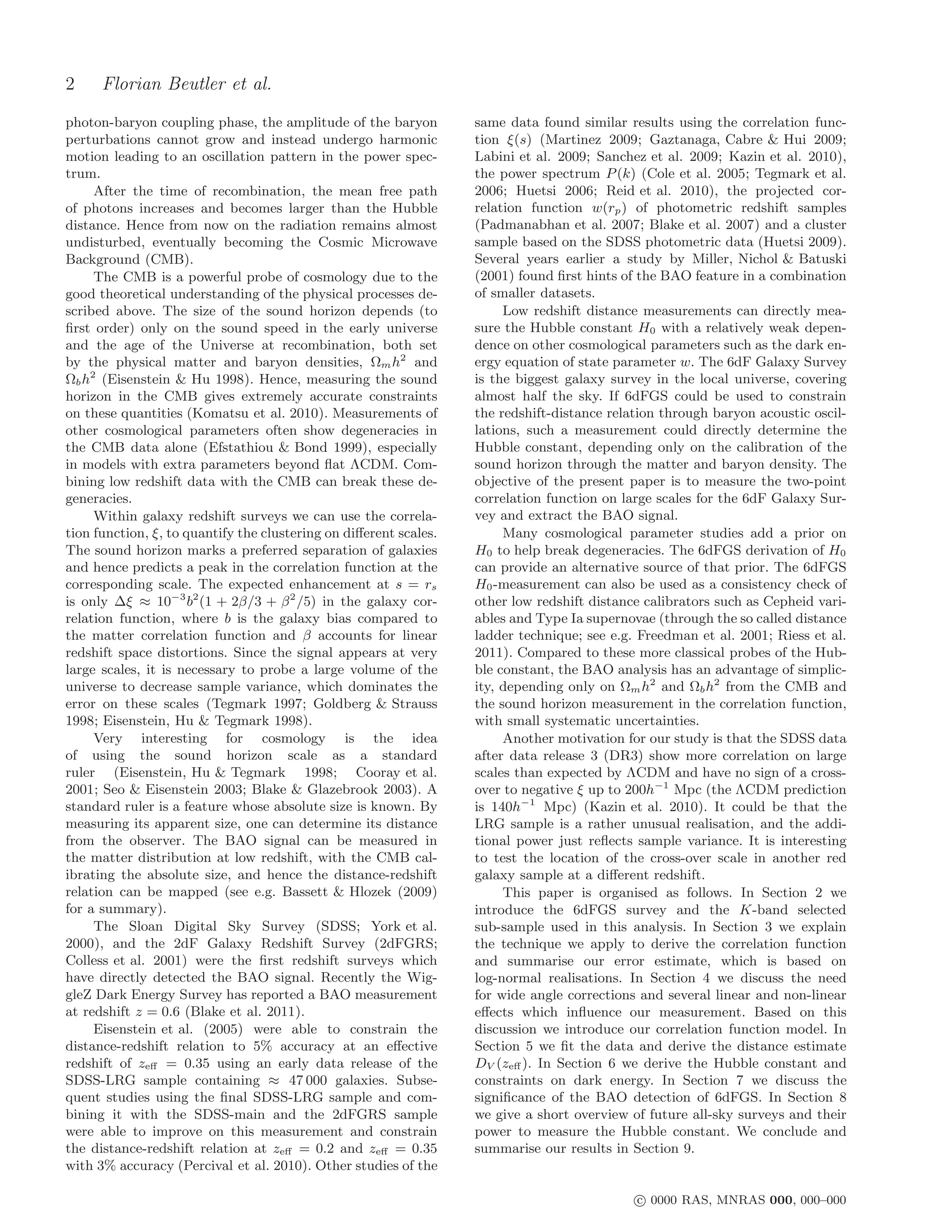
4. 4 Florian Beutler et al.
where the ratio nr /nd is given by
0.05 Nr
6dFGS data nr i wi (x)
= Nd
(5)
0.04 best fit nd j wj (x)
Ωmh2 = 0.12
0.03 Ωmh2 = 0.15 and the sums go over all random (Nr ) and data
no-baryon fit (Nd ) galaxies. We use the inverse density weighting
0.02 of Feldman, Kaiser & Peacock (1994):
ξ(s)
Ci
0.01 wi (x) = , (6)
1 + n(x)P0
0
with P0 = 40 000h3 Mpc−3 and Ci being the inverse com-
-0.01
pleteness weighting for 6dFGS (see Section 2.1 and Jones et
al., in preparation). This weighting is designed to minimise
-0.02 the error on the BAO measurement, and since our sample
20 40 60 80 100 120 140 160 180 200
s [h-1 Mpc] is strongly limited by sample variance on large scales this
weighting results in a significant improvement to the analy-
Figure 2. The large scale correlation function of 6dFGS. The sis. The effect of the weighting on the redshift distribution
best fit model is shown by the black line with the best fit value of is illustrated in Figure 1.
Ωm h2 = 0.138 ± 0.020. Models with different Ωm h2 are shown by Other authors have used the so called J3 -weighting
the green line (Ωm h2 = 0.12) and the blue line (Ωm h2 = 0.15). which optimises the error over all scales by weighting each
The red dashed line is a linear CDM model with Ωb h2 = 0 (and scale differently (e.g. Efstathiou 1988; Loveday et al. 1995).
Ωm h2 = 0.1), while all other models use the WMAP-7 best fit
In a magnitude limited sample there is a correlation be-
value of Ωb h2 = 0.02227 (Komatsu et al. 2010). The significance
of the BAO detection in the black line relative to the red dashed
tween luminosity and redshift, which establishes a correla-
line is 2.4σ (see Section 7). The error-bars at the data points tion between bias and redshift (Zehavi et al. 2005). A scale-
are the diagonal elements of the covariance matrix derived using dependent weighting would imply a different effective red-
log-normal mock catalogues. shift for each scale, causing a scale dependent bias.
Finally we considered a luminosity dependent weighting
as suggested by Percival, Verde & Peacock (2004). However
the same authors found that explicitly accounting for the
luminosity-redshift relation has a negligible effect for 2dF-
GRS. We found that the effect to the 6dFGS correlation
3.2 The correlation function function is ≪ 1σ for all bins. Hence the static weighting of
We turn the measured redshift into co-moving distance via eq. 6 is sufficient for our dataset.
We also include an integral constraint correction in the
z
c dz ′ form of
DC (z) = (2)
H0 0 E(z ′ ) ′
ξdata (s) = ξdata (s) + ic, (7)
with
where ic is defined as
E(z) = Ωfid (1 + z)3 + Ωfid (1 + z)2
m k
s RR(s)ξmodel (s)
fid 1/2 ic = . (8)
+ Ωfid (1 + z)3(1+w
Λ
)
) , (3) s RR(s)
where the curvature Ωfid is set to zero, the dark energy den-
k
The function RR(s) is calculated from our mock catalogue
sity is given by Ωfid = 1 − Ωfid and the equation of state for
Λ m and ξmodel (s) is a correlation function model. Since ic de-
dark energy is wfid = −1. Because of the very low redshift pends on the model of the correlation function we have to
of 6dFGS, our data are not very sensitive to Ωk , w or any re-calculate it at each step during the fitting procedure.
other higher dimensional parameter which influences the ex- However we note that ic has no significant impact to the
pansion history of the universe. We will discuss this further final result.
in Section 5.3. Figure 2 shows the correlation function of 6dFGS at
Now we measure the separation between all galaxy pairs large scales. The BAO peak at ≈ 105h−1 Mpc is clearly
in our survey and count the number of such pairs in each sep- visible. The plot includes model predictions of different cos-
aration bin. We do this for the 6dFGS data catalogue, a ran- mological parameter sets. We will discuss these models in
dom catalogue with the same selection function and a com- Section 5.2.
bination of data-random pairs. We call the pair-separation
distributions obtained from this analysis DD(s), RR(s) and
DR(s), respectively. The binning is chosen to be from 3.3 Log-normal error estimate
10h−1 Mpc up to 190h−1 Mpc, in 10h−1 Mpc steps. In the
To obtain reliable error-bars for the correlation function we
analysis we used 30 random catalogues with the same size as
use log-normal realisations (Coles & Jones 1991; Cole et al.
the data catalogue. The redshift correlation function itself
2005; Kitaura et al. 2009). In what follows we summarise
is given by Landy & Szalay (1993):
the main steps, but refer the interested reader to Ap-
2
′ DD(s) nr DR(s) nr pendix A in which we give a detailed explanation of how we
ξdata (s) = 1 + −2 , (4)
RR(s) nd RR(s) nd generate the log-normal mock catalogues. In Appendix B
c 0000 RAS, MNRAS 000, 000–000

5. 6dFGS: BAOs and the Local Hubble Constant 5
trix
N
200 1 ξn (si ) − ξ(si ) ξn (sj ) − ξ(sj )
Cij = . (11)
n=1
N −1
Here, ξn (si ) is the correlation function estimate at separa-
150 0.5 tion si and the sum goes over all N log-normal realisations.
The mean value is defined as
N
1
s [h-1Mpc]
ξ(ri ) = ξn (si ). (12)
N
100 0 n=1
The case i = j gives the error (ignoring correlations between
2
bins, σi = Cii ). In the following we will use this uncertainty
in all diagrams, while the fitting procedures use the full co-
50 -0.5
variance matrix.
The distribution of recovered correlation functions in-
cludes the effects of sample variance and shot noise. Non-
linearities are also approximately included since the distri-
0 -1
bution of over-densities is skewed.
0 50 100 150 200
s [h-1Mpc] In Figure 3 we show the log-normal correlation matrix
rij calculated from the covariance matrix. The correlation
Figure 3. Correlation matrix derived from a covariance matrix matrix is defined as
calculated from 200 log-normal realisations.
Cij
rij = , (13)
Cii Cjj
where C is the covariance matrix (for a comparison to jack-
knife errors see appendix B).
we compare the log-normal errors with jack-knife estimates.
Log-normal realisations of a galaxy survey are usually 4 MODELLING THE BAO SIGNAL
obtained by deriving a density field from a model power
spectrum, P (k), assuming Gaussian fluctuations. This den- In this section we will discuss wide-angle effects and non-
sity field is then Poisson sampled, taking into account the linearities. We also introduce a model for the large scale
window function and the total number of galaxies. The as- correlation function, which we later use to fit our data.
sumption that the input power spectrum has Gaussian fluc-
tuations can only be used in a model for a density field
with over-densities ≪ 1. As soon as we start to deal with 4.1 Wide angle formalism
finite rms fluctuations, the Gaussian model assigns a non- The model of linear redshift space distortions introduced
zero probability to regions of negative density. A log-normal by Kaiser (1987) is based on the plane parallel approxi-
random field LN (x), can avoid this unphysical behaviour. mation. Earlier surveys such as SDSS and 2dFGRS are at
It is obtained from a Gaussian field G(x) by sufficiently high redshift that the maximum opening an-
LN (x) = exp[G(x)] (9) gle between a galaxy pair remains small enough to en-
sure the plane parallel approximation is valid. However, the
which is positive-definite but approaches 1 + G(x) when- 6dF Galaxy Survey has a maximum opening angle of 180◦
ever the perturbations are small (e.g. at large scales). Cal- and a lower mean redshift of z ≈ 0.1 (for our weighted
culating the power spectrum of a Poisson sampled density sample) and so it is necessary to test the validity of the
field with such a distribution will reproduce the input power plane parallel approximation. The wide angle description
spectrum convolved with the window function. As an input of redshift space distortions has been laid out in several
power spectrum for the log-normal field we use papers (Szalay et al. 1997; Szapudi 2004; Matsubara 2004;
Papai & Szapudi 2008; Raccanelli et al. 2010), which we
Pnl (k) = APlin (k) exp[−(k/k∗ )2 ] (10)
summarise in Appendix C.
2 2
where A = b (1 + 2β/3 + β /5) accounts for the linear We find that the wide-angle corrections have only a very
bias and the linear redshift space distortions. Plin (k) is a minor effect on our sample. For our fiducial model we found a
linear model power spectrum in real space obtained from correction of ∆ξ = 4 · 10−4 in amplitude at s = 100h−1 Mpc
CAMB (Lewis et al. 2000) and Pnl (k) is the non-linear and ∆ξ = 4.5 · 10−4 at s = 200h−1 Mpc, (Figure C2 in
power spectrum in redshift space. Comparing the model the appendix). This is much smaller than the error bars on
above with the 6dFGS data gives A = 4. The damping pa- these scales. Despite the small size of the effect, we never-
rameter k∗ is set to k∗ = 0.33h Mpc−1 , as found in 6dFGS theless include all first order correction terms in our correla-
(see fitting results later). How well this input model matches tion function model. It is important to note that wide angle
the 6dFGS data can be seen in Figure 9. corrections affect the correlation function amplitude only
We produce 200 such realisations and calculate the cor- and do not cause any shift in the BAO scale. The effect of
relation function for each of them, deriving a covariance ma- the wide-angle correction on the unweighted sample is much
c 0000 RAS, MNRAS 000, 000–000

6. 6 Florian Beutler et al.
greater and is already noticeable on scales of 20h−1 Mpc. with the BAO oscillations predicted by linear theory. This
Weighting to higher redshifts mitigates the effect because it leads to shifts in the scale of oscillation nodes with re-
reduces the average opening angle between galaxy pairs, by spect to a smooth spectrum. In real space this corresponds
giving less weight to wide angle pairs (on average). to a peak shift towards smaller scales. Based on their re-
sults, Crocce & Scoccimarro (2008) propose a model to be
used for the correlation function analysis at large scales. We
4.2 Non-linear effects will introduce this model in the next section.
There are a number of non-linear effects which can poten-
tially influence a measurement of the BAO signal. These in-
clude scale-dependent bias, the non-linear growth of struc-
4.3 Large-scale correlation function
ture on smaller scales, and redshift space distortions. We
discuss each of these in the context of our 6dFGS sample. To model the correlation function on large scales, we fol-
As the universe evolves, the acoustic signature in the low Crocce & Scoccimarro (2008) and Sanchez et al. (2008)
correlation function is broadened by non-linear gravitational and adopt the following parametrisation1 :
structure formation. Equivalently we can say that the higher
∂ξ(s)
harmonics in the power spectrum, which represent smaller ξmodel (s) = B(s)b2 ξ(s) ∗ G(r) + ξ1 (r)
′ 1
. (14)
scales, are erased (Eisenstein, Seo & White 2007). ∂s
The early universe physics, which we discussed briefly in Here, we decouple the scale dependency of the bias B(s)
the introduction, is well understood and several authors have and the linear bias b. G(r) is a Gaussian damping term, ac-
produced software packages (e.g. CMBFAST and CAMB) counting for non-linear suppression of the BAO signal. ξ(s) is
and published fitting functions (e.g Eisenstein & Hu 1998) the linear correlation function (including wide angle descrip-
to make predictions for the correlation function and power tion of redshift space distortions; eq. C4 in the appendix).
spectrum using thermodynamical models of the early uni- The second term in eq 14 accounts for the mode-coupling of
verse. These models already include the basic linear physics different Fourier modes. It contains ∂ξ(s)/∂s, which is the
most relevant for the BAO peak. In our analysis we use first derivative of the redshift space correlation function, and
1
the CAMB software package (Lewis et al. 2000). The non- ξ1 (r), which is defined as
linear evolution of the power spectrum in CAMB is cal- ∞
1 1
culated using the halofit code (Smith et al. 2003). This ξ1 (r) = dk kPlin (k)j1 (rk), (15)
code is calibrated by n-body simulations and can describe 2π 2 0
non-linear effects in the shape of the matter power spec- with j1 (x) being the spherical Bessel function of order 1.
trum for pure CDM models to an accuracy of around Sanchez et al. (2008) used an additional parameter AMC
5 − 10% (Heitmann et al. 2010). However, it has previ- which multiplies the mode coupling term in equation 14.
ously been shown that this non-linear model is a poor We found that our data is not good enough to constrain
description of the non-linear effects around the BAO this parameter, and hence adopted AMC = 1 as in the orig-
peak (Crocce & Scoccimarro 2008). We therefore decided to inal model by Crocce & Scoccimarro (2008).
use the linear model output from CAMB and incorporate In practice we generate linear model power spectra
the non-linear effects separately. Plin (k) from CAMB and convert them into a correlation
All non-linear effects influencing the correlation func- function using a Hankel transform
tion can be approximated by a convolution with a Gaus- ∞
1
sian damping factor exp[−(rk∗ /2)2 ] (Eisenstein et al. 2007; ξ(r) = dk k2 Plin (k)j0 (rk), (16)
2π 2 0
Eisenstein, Seo & White 2007), where k∗ is the damping
scale. We will use this factor in our correlation function where j0 (x) = sin(x)/x is the spherical Bessel function of
model introduced in the next section. The convolution with order 0.
a Gaussian causes a shift of the peak position to larger scales, The ∗-symbol in eq. 14 is only equivalent to a convo-
since the correlation function is not symmetric around the lution in the case of a 3D correlation function, where we
peak. However this shift is usually very small. have the Fourier theorem relating the 3D power spectrum
All of the non-linear processes discussed so far are not to the correlation function. In case of the spherically aver-
at the fundamental scale of 105h−1 Mpc but are instead at aged quantities this is not true. Hence, the ∗-symbol in our
the cluster-formation scale of up to 10h−1 Mpc. The scale of equation stands for the multiplication of the power spectrum
105h−1 Mpc is far larger than any known non-linear effect in ˜
with G(k) before transforming it into a correlation function.
cosmology. This has led some authors to the conclusion that ˜
G(k) is defined as
the peak will not be shifted significantly, but rather only ˜
G(k) = exp −(k/k∗ )2 , (17)
blurred out. For example, Eisenstein, Seo & White (2007)
have argued that any systematic shift of the acoustic scale with the property
in real space must be small ( 0.5%), even at z = 0.
˜
G(k) → 0 as k → ∞. (18)
However, several authors report possible shifts of up
to 1% (Guzik & Bernstein 2007; Smith et al. 2008, 2007; The damping scale k∗ can be calculated from linear the-
Angulo et al. 2008). Crocce & Scoccimarro (2008) used re-
normalised perturbation theory (RPT) and found percent-
level shifts in the BAO peak. In addition to non-linear evo-
lution, they found that mode-coupling generates additional 1 note that r = s, the different letters just specify whether the
oscillations in the power spectrum, which are out of phase function is evaluated in redshift space or real space.
c 0000 RAS, MNRAS 000, 000–000

7. 6dFGS: BAOs and the Local Hubble Constant 7
Table 1. This table contains all parameter constraints from 5.1 Fitting preparation
6dFGS obtained in this paper. The priors used to derive these
parameters are listed in square brackets. All parameters as- The effective redshift of our sample is determined by
sume Ωb h2 = 0.02227 and in cases where a prior on Ωm h2 is Nb Nb
used, we adopt the WMAP-7 Markov chain probability distribu- wi wj
zeff = 2
(zi + zj ), (21)
tion (Komatsu et al. 2010). A(zeff ) is the acoustic parameter de- i j
2Nb
fined by Eisenstein et al. (2005) (see equation 27 in the text) and
R(zeff ) is the distance ratio of the 6dFGS BAO measurement to where Nb is the number of galaxies in a particular separa-
the last-scattering surface. The most sensible value for cosmolog- tion bin and wi and wj are the weights for those galaxies
ical parameter constraints is rs (zd )/DV (zeff ), since this measure- from eq. 6. We choose zeff from bin 10 which has the limits
ment is uncorrelated with Ωm h2 . The effective redshift of 6dFGS 100h−1 Mpc and 110h−1 Mpc and which gave zeff = 0.106.
is zeff = 0.106 and the fitting range is from 10 − 190h−1 Mpc. Other bins show values very similar to this, with a standard
deviation of ±0.001. The final result does not depend
Summary of parameter constraints from 6dFGS on a very precise determination of zeff , since we are not
Ωm h 2 0.138 ± 0.020 (14.5%) constraining a distance to the mean redshift, but a distance
DV (zeff ) 456 ± 27 Mpc (5.9%) ratio (see equation 24, later). In fact, if the fiducial model is
DV (zeff ) 459 ± 18 Mpc (3.9%) [Ωm h2 prior] correct, the result is completely independent of zeff . Only if
rs (zd )/DV (zeff ) 0.336 ± 0.015 (4.5%) there is a z-dependent deviation from the fiducial model do
R(zeff ) 0.0324 ± 0.0015 (4.6%) we need zeff to quantify this deviation at a specific redshift.
A(zeff ) 0.526 ± 0.028 (5.3%)
Ωm 0.296 ± 0.028 (9.5%) [Ωm h2 prior] Along the line-of-sight, the BAO signal directly con-
H0 67 ± 3.2 (4.8%) [Ωm h2 prior] strains the Hubble constant H(z) at redshift z. When mea-
sured in a redshift shell, it constrains the angular diameter
distance DA (z) (Matsubara 2004). In order to separately
measure DA (z) and H(z) we require a BAO detection in
the 2D correlation function, where it will appear as a ring
ory (Crocce & Scoccimarro 2006; Matsubara 2008) by at around 105h−1 Mpc. Extremely large volumes are neces-
sary for such a measurement. While there are studies that
∞ −1/2
1 report a successful (but very low signal-to-noise) detection in
k∗ = dk Plin (k) , (19)
6π 2 0
the 2D correlation function using the SDSS-LRG data (e.g.
Gaztanaga, Cabre & Hui 2009; Chuang & Wang 2011, but
where Plin (k) is again the linear power spectrum. ΛCDM
see also Kazin et al. 2010), our sample does not allow this
predicts a value of k∗ ≃ 0.17h Mpc−1 . However, we will
kind of analysis. Hence we restrict ourself to the 1D corre-
include k∗ as a free fitting parameter.
lation function, where we measure a combination of DA (z)
The scale dependance of the 6dFGS bias, B(s), is de- and H(z). What we actually measure is a superposition of
rived from the GiggleZ simulation (Poole et al., in prepara- two angular measurements (R.A. and Dec.) and one line-of-
tion); a dark matter simulation containing 21603 particles sight measurement (redshift). To account for this mixture of
in a 1h−1 Gpc box. We rank-order the halos of this simula- measurements it is common to report the BAO distance con-
tion by Vmax and choose a contiguous set of 250 000 of them, straints as (Eisenstein et al. 2005; Padmanabhan & White
selected to have the same clustering amplitude of 6dFGS as 2008)
quantified by the separation scale r0 , where ξ(r0 ) = 1. In
1/3
the case of 6dFGS we found r0 = 9.3h−1 Mpc. Using the cz
redshift space correlation function of these halos and of a DV (z) = (1 + z)2 DA (z)
2
, (22)
H0 E(z)
randomly subsampled set of ∼ 106 dark matter particles,
where DA is the angular distance, which in the case of Ωk =
we obtain
0 is given by DA (z) = DC (z)/(1 + z).
−1.332
B(s) = 1 + s/0.474h−1 Mpc , (20) To derive model power spectra from CAMB we have to
which describes a 1.7% correction of the correlation function specify a complete cosmological model, which in the case of
amplitude at separation scales of 10h−1 Mpc. To derive this the simplest ΛCDM model (Ωk = 0, w = −1), is specified
function, the GiggleZ correlation function (snapshot z = 0) by six parameters: ωc , ωb , ns , τ , As and h. These parame-
has been fitted down to 6h−1 Mpc, well below the smallest ters are: the physical cold dark matter and baryon density,
scales we are interested in. (ωc = Ωc h2 , ωb = Ωb h2 ), the scalar spectral index, (ns ), the
optical depth at recombination, (τ ), the scalar amplitude of
the CMB temperature fluctuation, (As ), and the Hubble
constant in units of 100 km s−1 Mpc−1 (h).
Our fit uses the parameter values from WMAP-
7 (Komatsu et al. 2010): Ωb h2 = 0.02227, τ = 0.085 and
ns = 0.966 (maximum likelihood values). The scalar ampli-
5 EXTRACTING THE BAO SIGNAL
tude As is set so that it results in σ8 = 0.8, which depends
In this section we fit the model correlation function devel- on Ωm h2 . However σ8 is degenerated with the bias parame-
oped in the previous section to our data. Such a fit can be ter b which is a free parameter in our fit. Furthermore, h is
used to derive the distance scale DV (zeff ) at the effective set to 0.7 in the fiducial model, but can vary freely in our
redshift of the survey. fit through a scale distortion parameter α, which enters the
c 0000 RAS, MNRAS 000, 000–000

8. 8 Florian Beutler et al.
600 6dFGS
constant Γ = Ωmh 1.1 Percival et al. (2009)
constant rs/DV ΛCDM (fiducial)
fid
DV (z) = cz/H
550 fiducial model 0
1.05
best fit
1.2
HfidDV(z)/cz
DV (z = 0.106) [Mpc]
500 1
0
0.95
α
450
1
0.9
400
0.85
0 0.05 0.1 0.15 0.2 0.25 0.3 0.35 0.4
0.8 z
350
Figure 5. The distance measurement DV (z) relative to a low
0.05 0.1 0.15 0.2 redshift approximation. The points show 6dFGS data and those
Ωmh2 of Percival et al. (2010).
Figure 4. Likelihood contours of the distance DV (zeff ) against
Ωm h2 . The corresponding values of α are given on the right-hand
axis. The contours show 1 and 2σ errors for both a full fit (blue linearities is not good enough to capture the effects on such
solid contours) and a fit over 20 − 190h−1 Mpc (black dashed scales. The upper limit is chosen to be well above the BAO
contours) excluding the first data point. The black cross marks scale, although the constraining contribution of the bins
the best fitting values corresponding to the dashed black contours above 130h−1 Mpc is very small. Our final model has 4 free
with (DV , Ωm h2 ) = (462, 0.129), while the blue cross marks the parameters: Ωm h2 , b, α and k∗ .
best fitting values for the blue contours. The black solid curve The best fit corresponds to a minimum χ2 of 15.7 with
corresponds to a constant Ωm h2 DV (zeff ) (DV ∼ h−1 ), while the
14 degrees of freedom (18 data-points and 4 free parame-
dashed line corresponds to a constant angular size of the sound
ters). The best fitting model is included in Figure 2 (black
horizon, as described in the text.
line). The parameter values are Ωm h2 = 0.138 ± 0.020,
b = 1.81 ± 0.13 and α = 1.036 ± 0.062, where the er-
rors are derived for each parameter by marginalising over
model as all other parameters. For k∗ we can give a lower limit of
′
ξmodel (s) = ξmodel (αs). (23) k∗ = 0.19h Mpc−1 (with 95% confidence level).
We can use eq. 24 to turn the measurement of α into
This parameter accounts for deviations from the fiducial cos- a measurement of the distance to the effective redshift
mological model, which we use to derive distances from the fid
DV (zeff ) = αDV (zeff ) = 456 ± 27 Mpc, with a precision
measured redshift. It is defined as (Eisenstein et al. 2005; fid
of 5.9%. Our fiducial model gives DV (zeff ) = 440.5 Mpc,
Padmanabhan & White 2008) where we have followed the distance definitions of Wright
DV (zeff ) (2006) throughout. For each fit we derive the parameter
α= fid
. (24) β = Ωm (z)0.545 /b, which we need to calculate the wide angle
DV (zeff )
corrections for the correlation function.
The parameter α enables us to fit the correlation function The maximum likelihood distribution of k∗ seems to
derived with the fiducial model, without the need to re- prefer smaller values than predicted by ΛCDM, although
calculate the correlation function for every new cosmological we are not able to constrain this parameter very well. This
parameter set. is connected to the high significance of the BAO peak in the
At low redshift we can approximate H(z) ≈ H0 , which 6dFGS data (see Section 7). A smaller value of k∗ damps the
results in BAO peak and weakens the distance constraint. For compar-
fid
H0 ison we also performed a fit fixing k∗ to the ΛCDM predic-
α≈ . (25) tion of k∗ ≃ 0.17h Mpc−1 . We found that the error on the
H0
distance DV (zeff ) increases from 5.9% to 8%. However since
Compared to the correct equation 24 this approximation
the data do not seem to support such a small value of k∗ we
has an error of about 3% at redshift z = 0.1 for our fiducial
prefer to marginalise over this parameter.
model. Since this is a significant systematic bias, we do not
The contours of DV (zeff )−Ωm h2 are shown in Figure 4,
use this approximation at any point in our analysis.
together with two degeneracy predictions (Eisenstein et al.
2005). The solid line is that of constant Ωm h2 DV (zeff ),
which gives the direction of degeneracy for a pure CDM
5.2 Extracting DV (zeff ) and rs (zd )/DV (zeff )
model, where only the shape of the correlation function
Using the model introduced above we performed fits to 18 contributes to the fit, without a BAO peak. The dashed
data points between 10h−1 Mpc and 190h−1 Mpc. We ex- line corresponds to a constant rs (zd )/DV (zeff ), which is the
cluded the data below 10h−1 Mpc, since our model for non- degeneracy if only the position of the acoustic scale con-
c 0000 RAS, MNRAS 000, 000–000

9. 6dFGS: BAOs and the Local Hubble Constant 9
tributes to the fit. The dashed contours exclude the first Focusing on the path from z = 0 to zeff = 0.106, our
data point, fitting from 20 − 190h−1 Mpc only, with the dataset can give interesting constraints on Ωm . We derive
best fitting values α = 1.049 ± 0.071 (corresponding to the parameter (Eisenstein et al. 2005)
DV (zeff ) = 462 ± 31 Mpc), Ωm h2 = 0.129 ± 0.025 and √
Ωm h2
b = 1.72 ± 0.17. The contours of this fit are tilted towards A(zeff ) = 100DV (zeff ) , (27)
the dashed line, which means that the fit is now driven by czeff
the BAO peak, while the general fit (solid contours) seems which has no dependence on the Hubble constant since
to have some contribution from the shape of the correlation DV ∝ h−1 . We obtain A(zeff ) = 0.526 ± 0.028 with
function. Excluding the first data point increases the error χ2 /d.o.f. = 15.7/14. The value of A would be identical to
√
on the distance constraint only slightly from 5.9% to 6.8%. Ωm if measured at redshift z = 0. At redshift zeff = 0.106
The value of Ωm h2 tends to be smaller, but agrees within we obtain a deviation from this approximation of 6% for
1σ with the former value. our fiducial model, which is small but systematic. We can
Going back to the complete fit from 10 − 190h−1 Mpc, express A, including the curvature term Ωk and the dark
we can include an external prior on Ωm h2 from WMAP-7, energy equation of state parameter w, as
which carries an error of only 4% (compared to the ≈ 15% √
 sinh Ωk χ(z) 2/3

we obtain by fitting our data). Marginalising over Ωm h2 now 
 √ Ωk > 0
√ Ωk z

gives DV (zeff ) = 459 ± 18 Mpc, which reduces the error


Ωm 2/3

from 5.9% to 3.9%. The uncertainty in Ωm h2 from WMAP- A(z) = χ(z)
Ωk = 0 (28)
E(z)1/3  z √
7 contributes only about 5% of the error in DV (assuming no 

 sin |Ωk |χ(z) 2/3
error in the WMAP-7 value of Ωm h2 results in DV (zeff ) = √ Ωk < 0



|Ωk |z
459 ± 17 Mpc).
low−z
In Figure 5 we plot the ratio DV (z)/DV (z) as a with
low−z
function of redshift, where DV (z) = cz/H0 . At suffi- H0 z
dz ′
ciently low redshift the approximation H(z) ≈ H0 is valid χ(z) = DC (z) = (29)
c 0 E(z ′ )
and the measurement is independent of any cosmological
parameter except the Hubble constant. This figure also con- and
tains the results from Percival et al. (2010). E(z) = Ωm (1 + z)3 + Ωk (1 + z)2
Rather than including the WMAP-7 prior on Ωm h2 to
1/2
break the degeneracy between Ωm h2 and the distance con- + ΩΛ (1 + z)3(1+w) ) . (30)
straint, we can fit the ratio rs (zd )/DV (zeff ), where rs (zd ) is
Using this equation we now linearise our result for Ωm in Ωk
the sound horizon at the baryon drag epoch zd . In princi-
and w and get
ple, this is rotating Figure 4 so that the dashed black line
is parallel to the x-axis and hence breaks the degeneracy if Ωm = 0.287 + 0.039(1 + w) + 0.039Ωk ± 0.027. (31)
the fit is driven by the BAO peak; it will be less efficient
For comparison, Eisenstein et al. (2005) found
if the fit is driven by the shape of the correlation function.
During the fit we calculate rs (zd ) using the fitting formula Ωm = 0.273 + 0.123(1 + w) + 0.137Ωk ± 0.025 (32)
of Eisenstein & Hu (1998).
The best fit results in rs (zd )/DV (zeff ) = 0.336 ± 0.015, based on the SDSS LRG DR3 sample. This result shows the
which has an error of 4.5%, smaller than the 5.9% found reduced sensitivity of the 6dFGS measurement to w and Ωk .
for DV but larger than the error in DV when adding the
WMAP-7 prior on Ωm h2 . This is caused by the small dis-
agreement in the DV − Ωm h2 degeneracy and the line of 6 COSMOLOGICAL IMPLICATIONS
constant sound horizon in Figure 4. The χ2 is 15.7, simi-
lar to the previous fit with the same number of degrees of In this section we compare our results to other studies and
freedom. discuss the implications for constraints on cosmological pa-
rameters. We first note that we do not see any excess cor-
relation on large scales as found in the SDSS-LRG sample.
5.3 Extracting A(zeff ) and R(zeff ) Our correlation function is in agreement with a crossover to
negative scales at 140h−1 Mpc, as predicted from ΛCDM.
We can also fit for the ratio of the distance between the
effective redshift, zeff , and the redshift of decoupling (z∗ =
1091; Eisenstein et al. 2005);
6.1 Constraining the Hubble constant, H0
DV (zeff )
R(zeff ) = , (26) We now use the 6dFGS data to derive an estimate of
(1 + z∗ )DA (z∗ )
the Hubble constant. We use the 6dFGS measurement of
with (1 + z∗ )DA (z∗ ) being the CMB angular comoving dis- rs (zd )/DV (0.106) = 0.336 ± 0.015 and fit directly for the
tance. Beside the fact that the Hubble constant H0 can- Hubble constant and Ωm . We combine our measurement
cels out in the determination of R, this ratio is also more with a prior on Ωm h2 coming from the WMAP-7 Markov
robust against effects caused by possible extra relativistic chain results (Komatsu et al. 2010). Combining the cluster-
species (Eisenstein & White 2004). We calculate DA (z∗ ) for ing measurement with Ωm h2 from the CMB corresponds to
each Ωm h2 during the fit and then marginalise over Ωm h2 . the calibration of the standard ruler.
The best fit results in R = 0.0324 ± 0.0015, with χ2 = 15.7 We obtain values of H0 = 67±3.2 km s−1 Mpc−1 (which
and the same 14 degrees of freedom. has an uncertainty of only 4.8%) and Ωm = 0.296 ± 0.028.
c 0000 RAS, MNRAS 000, 000–000

10. 10 Florian Beutler et al.
Table 2. wCDM constraints from different datasets. Comparing the two columns shows the influence of the 6dFGS data point. The
6dFGS data point reduces the error on w by 24% compared to WMAP-7+LRG which contains only the BAO data points of Percival et al.
(2010). We assume flat priors of 0.11 < Ωm h2 < 0.16 and marginalise over Ωm h2 . The asterisks denote the free parameters in each fit.
parameter WMAP-7+LRG WMAP-7+LRG+6dFGS
H0 69.9 ± 3.8(*) 68.7 ± 2.8(*)
Ωm 0.283 ± 0.033 0.293 ± 0.027
ΩΛ 0.717 ± 0.033 0.707 ± 0.027
w -1.01 ± 0.17(*) -0.97 ± 0.13(*)
Table 3. Parameter constraints from WMAP7+BAO for (i) a flat ΛCDM model, (ii) an open ΛCDM (oΛCDM), (iii) a flat model
with w = const. (wCDM), and (iv) an open model with w = constant (owCDM). We assume flat priors of 0.11 < Ωm h2 < 0.16 and
marginalise over Ωm h2 . The asterisks denote the free parameters in each fit.
parameter ΛCDM oΛCDM wCDM owCDM
H0 69.2 ± 1.1(*) 68.3 ± 1.7(*) 68.7 ± 2.8(*) 70.4 ± 4.3(*)
Ωm 0.288 ± 0.011 0.290 ± 0.019 0.293 ± 0.027 0.274 ± 0.035
Ωk (0) -0.0036 ± 0.0060(*) (0) -0.013 ± 0.010(*)
ΩΛ 0.712 ± 0.011 0.714 ± 0.020 0.707 ± 0.027 0.726 ± 0.036
w (-1) (-1) -0.97 ± 0.13(*) -1.24 ± 0.39(*)
80
70
75
H0 [km s-1Mpc-1]
H0 [km s-1Mpc-1]
70
60
65
BAO
6dFGS WMAP-7
60
50 Ωmh2 prior BAO+WMAP-7
6dFGS + Ωmh2 prior without 6dFGS
55
0.15 0.2 0.25 0.3 0.35 0.4 -1.5 -1 -0.5
Ωm w
Figure 6. The blue contours show the WMAP-7 Ωm h2 Figure 7. The blue contours shows the WMAP-7 degeneracy in
prior (Komatsu et al. 2010). The black contour shows con- H0 and w (Komatsu et al. 2010), highlighting the need for a sec-
straints from 6dFGS derived by fitting to the measurement of ond dataset to break the degeneracy. The black contours show
rs (zd )/DV (zeff ). The solid red contours show the combined con- constraints from BAO data incorporating the rs (zd )/DV (zeff )
straints resulting in H0 = 67 ± 3.2 km s−1 Mpc−1 and Ωm = measurements of Percival et al. (2010) and 6dFGS. The solid
0.296 ± 0.028. Combining the clustering measurement with Ωm h2 red contours show the combined constraints resulting in w =
from the CMB corresponds to the calibration of the standard −0.97 ± 0.13. Excluding the 6dFGS data point widens the con-
ruler. straints to the dashed red line with w = −1.01 ± 0.17.
Table 1 and Figure 6 summarise the results. The value of
Ωm agrees with the value we derived earlier (Section 5.3). the shift parameter
To combine our measurement with the latest CMB data √
we use the WMAP-7 distance priors, namely the acoustic Ωm h2
R = 100 (1 + z∗ )DA (z∗ ) (34)
scale c
πDA (z∗ ) and the redshift of decoupling z∗ (Tables 9 and 10
ℓA = (1 + z∗ ) , (33) in Komatsu et al. 2010). This combined analysis reduces
rs (z∗ )
c 0000 RAS, MNRAS 000, 000–000

11. 6dFGS: BAOs and the Local Hubble Constant 11
the error further and yields H0 = 68.7 ± 1.5 km s−1 Mpc−1
(2.2%) and Ωm = 0.29 ± 0.022 (7.6%). 24
Percival et al. (2010) determine a value of H0 = 22
68.6 ± 2.2 km s−1 Mpc−1 using SDSS-DR7, SDSS-LRG and 20 6dFGS
2dFGRS, while Reid et al. (2010) found H0 = 69.4 ± 18
1.6 km s−1 Mpc−1 using the SDSS-LRG sample and WMAP- 16
5. In contrast to these results, 6dFGS is less affected by 14
N( ∆χ2)
parameters like Ωk and w because of its lower redshift. In 12
any case, our result of the Hubble constant agrees very
10
well with earlier BAO analyses. Furthermore our result
8
agrees with the latest CMB measurement of H0 = 70.3 ±
6
2.5 km s−1 Mpc−1 (Komatsu et al. 2010).
4
The SH0ES program (Riess et al. 2011) determined the
2
Hubble constant using the distance ladder method. They
0
used about 600 near-IR observations of Cepheids in eight 0 0.5 1 1.5 2 2.5 3 3.5 4
∆χ2
galaxies to improve the calibration of 240 low redshift
(z < 0.1) SN Ia, and calibrated the Cepheid distances us-
Figure 8. The number of log-normal realisations found with a
ing the geometric distance to the maser galaxy NGC 4258.
certain ∆χ2 , where the ∆χ2 is obtained by comparing a fit us-
They found H0 = 73.8 ± 2.4 km s−1 Mpc−1 , a value con- ing a ΛCDM correlation function model with a no-baryon model.
sistent with the initial results of the Hubble Key project The blue line indicates the 6dFGS result.
Freedman et al. (H0 = 72±8 km s−1 Mpc−1 ; 2001) but 1.7σ
higher than our value (and 1.8σ higher when we combine
our dataset with WMAP-7). While this could point toward
unaccounted or under-estimated systematic errors in either 250
one of the methods, the likelihood of such a deviation by Input
chance is about 10% and hence is not enough to represent a 200 6dFGS
significant discrepancy. Possible systematic errors affecting mean
150
the BAO measurements are the modelling of non-linearities,
bias and redshift-space distortions, although these system- 100
atics are not expected to be significant at the large scales
s2ξ(s)
50
relevant to our analysis.
To summarise the finding of this section we can state 0
that our measurement of the Hubble constant is competitive
-50
with the latest result of the distance ladder method. The dif-
ferent techniques employed to derive these results have very -100
different potential systematic errors. Furthermore we found
that BAO studies provide the most accurate measurement -150
0 20 40 60 80 100 120 140 160 180 200
of H0 that exists, when combined with the CMB distance s [h-1 Mpc]
priors.
Figure 9. The different log-normal realisations used to calculate
the covariance matrix (shown in grey). The red points indicate
6.2 Constraining dark energy the mean values, while the blue points show actual 6dFGS data
(the data point at 5h−1 Mpc is not included in the fit). The red
One key problem driving current cosmology is the determi- data points are shifted by 2h−1 Mpc to the right for clarity.
nation of the dark energy equation of state parameter, w.
When adding additional parameters like w to ΛCDM we find
large degeneracies in the WMAP-7-only data. One example The best fit gives w = −0.97 ± 0.13, H0 = 68.7 ±
is shown in Figure 7. WMAP-7 alone can not constrain H0 2.8 km s−1 Mpc−1 and Ωm h2 = 0.1380 ± 0.0055, with a
or w within sensible physical boundaries (e.g. w < −1/3). As χ2 /d.o.f. = 1.3/3. Table 2 and Figure 7 summarise the re-
we are sensitive to H0 , we can break the degeneracy between sults. To illustrate the importance of the 6dFGS result to
w and H0 inherent in the CMB-only data. Our assumption the overall fit we also show how the results change if 6dFGS
of a fiducial cosmology with w = −1 does not introduce a is omitted. The 6dFGS data improve the constraint on w by
bias, since our data is not sensitive to this parameter and 24%.
any deviation from this assumption is modelled within the Finally we show the best fitting cosmological parame-
shift parameter α. ters for different cosmological models using WMAP-7 and
We again use the WMAP-7 distance priors intro- BAO results in Table 3.
duced in the last section. In addition to our value of
rs (zd )/DV (0.106) = 0.336 ± 0.015 we use the results
of Percival et al. (2010), who found rs (zd )/DV (0.2) =
7 SIGNIFICANCE OF THE BAO DETECTION
0.1905 ± 0.0061 and rs (zd )/DV (0.35) = 0.1097 ± 0.0036.
To account for the correlation between the two latter data To test the significance of our detection of the BAO sig-
points we employ the covariance matrix reported in their nature we follow Eisenstein et al. (2005) and perform a fit
paper. Our fit has 3 free parameters, Ωm h2 , H0 and w. with a fixed Ωb = 0, which corresponds to a pure CDM
c 0000 RAS, MNRAS 000, 000–000

12. 12 Florian Beutler et al.
10000
6dFGS
30 WALLABY
TAIPAN1 (r < 17)
8000
25 TAIPAN2 (r < 16.5)
20 6000
n(z)
N
15
4000
10
2000
5
0 0
0.7 0.8 0.9 1 1.1 1.2 1.3 0 0.02 0.04 0.06 0.08 0.1 0.12 0.14 0.16 0.18 0.2
α z
Figure 10. This plot shows the distribution of the parameter α Figure 11. Redshift distribution of 6dFGS, WALLABY and two
derived from the 200 log-normal realisations (black). The distri- different versions of the proposed TAIPAN survey. See text for
bution is well fit by a Gaussian with a mean of µ = 0.998 ± 0.004 details.
and a width of σ = 0.057 ± 0.005. In blue we show the same dis-
tribution selecting only the log-normal realisations with a strong
BAO peak (> 2σ). The Gaussian distribution in this case gives a
very well with the data (with a reduced χ2 of 1.12) and is
mean of 1.007 ± 0.007 and σ = 0.041 ± 0.008.
within the range spanned by our log-normal realisations, we
can not claim any discrepancy with ΛCDM. Therefore, the
most likely explanation for the excess correlation in the BAO
model without a BAO signature. The best fit has χ2 = 21.4 peak is sample variance.
with 14 degrees of freedom and is shown as the red dashed In Figure 10 we show the distribution of the parameter
line in Figure 2. The parameter values of this fit depend on α obtained from the 200 log-normal realisations. The dis-
the parameter priors, which we set to 0.7 < α < 1.3 and tribution is well described by a Gaussian with χ2 /d.o.f. =
0.1 < Ωm h2 < 0.2. Values of α much further away from 14.2/20, where we employed Poisson errors for each bin.
1 are problematic since eq. 24 is only valid for α close to This confirms that α has Gaussian distributed errors in the
1. Comparing the best pure CDM model with our previous approximation that the 6dFGS sample is well-described by
fit, we estimate that the BAO signal is detected with a sig- log-normal realisations of an underlying ΛCDM power spec-
nificance of 2.4σ (corresponding to ∆χ2 = 5.6). As a more trum. This result increases our confidence that the appli-
qualitative argument for the detection of the BAO signal we cation of Gaussian errors for the cosmological parameter
would like to refer again to Figure 4 where the direction of fits is correct. The mean of the Gaussian distribution is at
the degeneracy clearly indicates the sensitivity to the BAO 0.998 ± 0.004 in agreement with unity, which shows, that we
peak. are able to recover the input model. The width of the dis-
We can also use the log-normal realisations to deter- tribution shows the mean expected error in α in a ΛCDM
mine how likely it is to find a BAO detection in a survey universe for a 6dFGS-like survey. We found σ = 0.057±0.005
like 6dFGS. To do this, we produced 200 log-normal mock which is in agreement with our error in α of 5.9%. Figure 10
catalogues and calculated the correlation function for each also contains the distribution of α, selecting only the log-
of them. We can now fit our correlation function model to normal realisations with a strong (> 2σ) BAO peak (blue
these realisations. Furthermore, we fit a no-baryon model to data). We included this selection to show, that a stronger
the correlation function and calculate ∆χ2 , the distribution BAO peak does not bias the estimate of α in any direc-
of which is shown in Figure 8. We find that 26% of all re- tion. The Gaussian fit gives χ2 /d.o.f. = 5/11 with a mean of
alisations have at least a 2σ BAO detection, and that 12% 1.007 ± 0.007. The distribution of α shows a smaller spread
have a detection > 2.4σ. The log-normal realisations show a with σ = 0.041 ± 0.008, about 2σ below our error on α. This
mean significance of the BAO detection of 1.7 ± 0.7σ, where result shows, that a survey like 6dFGS is able to constrain
the error describes the variance around the mean. α (and hence DV and H0 ) to the precision we report in this
Figure 9 shows the 6dFGS data points together with paper.
all 200 log-normal realisations (grey). The red data points
indicate the mean for each bin and the black line is the input
model derived as explained in Section 3.3. This comparison
shows that the 6dFGS data contain a BAO peak slightly 8 FUTURE ALL SKY SURVEYS
larger than expected in ΛCDM. A major new wide-sky survey of the local Universe will be
The amplitude of the acoustic feature relative to the Wide field ASKAP L-band Legacy All-sky Blind surveY
the overall normalisation of the galaxy correlation func- (WALLABY)2 . This is a blind HI survey planned for the
tion is quite sensitive to the baryon fraction, fb = Australian SKA Pathfinder telescope (ASKAP), currently
Ωb /Ωm (Matsubara 2004). A higher BAO peak could hence
point towards a larger baryon fraction in the local universe.
However since the correlation function model seems to agree 2 http://www.atnf.csiro.au/research/WALLABY
c 0000 RAS, MNRAS 000, 000–000

13. 6dFGS: BAOs and the Local Hubble Constant 13
The TAIPAN survey3 proposed for the UK Schmidt
150 Telescope at Siding Spring Observatory, will cover a com-
TAIPAN1
parable area of sky, and will extend 6dFGS in both depth
TAIPAN2
Input and redshift (z ≃ 0.08).
100
The redshift distribution of both surveys is shown in
Figure 11, alongside 6dFGS. Since the TAIPAN survey is
50 still in the early planning stage we consider two realisa-
s2ξ(s)
tions: TAIPAN1 (406 000 galaxies to a faint magnitude limit
of r = 17) and the shallower TAIPAN2 (221 000 galax-
0 ies to r = 16.5). We have adopted the same survey win-
dow as was used for 6dFGS, meaning that it covers the
whole southern sky excluding a 10◦ strip around the Galac-
-50
tic plane. The effective volumes of TAIPAN1 and TAIPAN2
are 0.23h−3 Gpc3 and 0.13h−3 Gpc3 , respectively.
20 40 60 80 100 120 140 160 180 200 To predict the ability of these surveys to measure the
s [h-1 Mpc]
large scale correlation function we produced 100 log-normal
realisations for TAIPAN1 and WALLABY and 200 log-
Figure 12. Predictions for two versions of the proposed TAIPAN
survey. Both predictions assume a 2π steradian southern sky-
normal realisations for TAIPAN2. Figures 12 and 13 show
coverage, excluding the Galactic plane (i.e. |b| > 10◦ ). TAIPAN1 the results in each case. The data points are the mean of
contains 406 000 galaxies while TAIPAN2 contains 221 000, (see the different realisations, and the error bars are the diago-
Figure 11). The blue points are shifted by 2h−1 Mpc to the right nal of the covariance matrix. The black line represents the
for clarity. The black line is the input model, which is a ΛCDM input model which is a ΛCDM prediction convolved with
model with a bias of 1.6, β = 0.3 and k∗ = 0.17h Mpc−1 . For a Gaussian damping term using k∗ = 0.17h Mpc−1 (see
a large number of realisations, the difference between the input eq. 17). We used a bias parameter of 1.6 for TAIPAN and
model and the mean (the data points) is only the convolution following our fiducial model we get β = 0.3, resulting in
with the window function. A = b2 (1 + 2β/3 + β 2 /5) = 3.1. For WALLABY we used a
bias of 0.7 (based on the results found in the HIPASS sur-
vey; Basilakos et al. 2007). This results in β = 0.7 and
A = 0.76. To calculate the correlation function we used
WALLABY P0 = 40 000h3 Mpc3 for TAIPAN and P0 = 5 000h3 Mpc3
25 for WALLABY.
Input
20 The error bar for TAIPAN1 is smaller by roughly a fac-
15 tor of 1.7 relative to 6dFGS, which is consistent with scal-
√
ing by Veff and is comparable to the SDSS-LRG sample.
10
We calculate the significance of the BAO detection for each
s2ξ(s)
5 log-normal realisation by performing fits to the correlation
0 function using ΛCDM parameters and Ωb = 0, in exactly
the same manner as the 6dFGS analysis described earlier.
-5
We find a 3.5 ± 0.8σ significance for the BAO detection for
-10 TAIPAN1, 2.1 ± 0.7σ for TAIPAN2 and 2.1 ± 0.7σ for WAL-
-15 LABY, where the error again describes the variance around
-20
the mean.
20 40 60 80 100 120 140 160 180 200 We then fit a correlation function model to the mean
s [h-1 Mpc]
values of the log-normal realisations for each survey, using
Figure 13. Prediction for the WALLABY survey. We have as- the covariance matrix derived from these log-normal real-
sumed a 4π steradian survey with 602 000 galaxies, b = 0.7, isations. We evaluated the correlation function of WAL-
β = 0.7 and k∗ = 0.17h Mpc−1 . LABY, TAIPAN2 and TAIPAN1 at the effective redshifts
of 0.1, 0.12 and 0.14, respectively. With these in hand, we
are able to derive distance constraints to respective preci-
under construction at the Murchison Radio-astronomy Ob- sions of 7%, 6% and 3%. The predicted value for WAL-
servatory (MRO) in Western Australia. LABY is not significantly better than that from 6dFGS.
The survey will cover at least 75% of the sky with the This is due to the significance of the 6dFGS BAO peak in
potential to cover 4π of sky if the Westerbork Radio Tele- the data, allowing us to place tight constraints on the dis-
scope delivers complementary northern coverage. Compared tance. As an alternative figure-of-merit, we derive the con-
to 6dFGS, WALLABY will more than double the sky cov- straints on the Hubble constant. All surveys recover the in-
erage including the Galactic plane. WALLABY will contain put parameter of H0 = 70 km s−1 Mpc−1 , with absolute un-
∼ 500 000 to 600 000 galaxies with a mean redshift of around certainties of 3.7, 3 and 2.2 km s−1 Mpc−1 for WALLABY,
0.04, giving it around 4 times greater galaxy density com- TAIPAN2 and TAIPAN1, respectively. Hence, TAIPAN1 is
pared to 6dFGS. In the calculations that follow, we assume
for WALLABY a 4π survey without any exclusion around
the Galactic plane. The effective volume in this case turns 3 TAIPAN: Transforming Astronomical Imaging surveys through
out to be 0.12h−3 Gpc3 . Polychromatic Analysis of Nebulae
c 0000 RAS, MNRAS 000, 000–000

14. 14 Florian Beutler et al.
able to constrain the Hubble constant to 3% precision. These • We are able to measure the Hubble constant, H0 =
constraints might improve when combined with Planck con- 67 ± 3.2 km s−1 Mpc−1 , to 4.8% precision, using only the
straints on Ωb h2 and Ωm h2 which will be available when standard ruler calibration by the CMB (in form of Ωm h2 and
these surveys come along. Ωb h2 ). Compared to previous BAO measurements, 6dFGS is
Since there is significant overlap between the survey almost completely independent of cosmological parameters
volume of 6dFGS, TAIPAN and WALLABY, it might be (e.g. Ωk and w), similar to Cepheid and low-z supernovae
interesting to test whether the BAO analysis of the local methods. However, in contrast to these methods, the BAO
universe can make use of a multiple tracer analysis, as sug- derivation of the Hubble constant depends on very basic
gested recently by Arnalte-Mur et al. (2011). These authors early universe physics and avoids possible systematic errors
claim that by employing two different tracers of the matter coming from the build up of a distance ladder.
density field – one with high bias to trace the central over- • By combining the 6dFGS BAO measurement with those
densities, and one with low bias to trace the small density of WMAP-7 and previous redshift samples Percival et al.
fluctuations – one can improve the detection and measure- (from SDSS-DR7, SDDS-LRG and 2dFGRS; 2010), we can
ment of the BAO signal. Arnalte-Mur et al. (2011) test this further improve the constraints on the dark energy equation
approach using the SDSS-LRG sample (with a very large of state, w, by breaking the H0 − w degeneracy in the CMB
bias) and the SDSS-main sample (with a low bias). Although data. Doing this, we find w = −0.97 ± 0.13, which is an
the volume is limited by the amount of sample overlap, they improvement of 24% compared to previous combinations of
detect the BAO peak at 4.1σ. Likewise, we expect that the BAO and WMAP-7 data.
contrasting high bias of 6dFGS and TAIPAN, when used in • We have made detailed predictions for two next-
conjunction with the low bias of WALLABY, would furnish generation low redshift surveys, WALLABY and TAIPAN.
a combined sample that would be ideal for such an analysis. Using our 6dFGS result, we predict that both surveys will
Neither TAIPAN nor WALLABY are designed as BAO detect the BAO signal, and that WALLABY may be the first
surveys, with their primary goals relating to galaxy forma- radio galaxy survey to do so. Furthermore, we predict that
tion and the local universe. However, we have found that TAIPAN has the potential to constrain the Hubble constant
TAIPAN1 would be able to improve the measurement of the to a precision of 3% improving the 6dFGS measurement by
local Hubble constant by about 30% compared to 6dFGS go- 30%.
ing to only slightly higher redshift. WALLABY could make
some interesting contributions in the form of a multiple
tracer analysis.
ACKNOWLEDGMENTS
The authors thank Alex Merson for providing the random
9 CONCLUSION mock generator and Lado Samushia for helpful advice with
the wide-angle formalism. We thank Martin Meyer and
We have calculated the large-scale correlation function of the Alan Duffy for fruitful discussions and Greg Poole for pro-
6dF Galaxy Survey and detected a BAO peak with a sig- viding the relation for the scale dependent bias. We also
nificance of 2.4σ. Although 6dFGS was never designed as a thank Tamara Davis, Eyal Kazin and John Peacock for com-
BAO survey, the peak is detectable because the survey con- ments on earlier versions of this paper. F.B. is supported
tains a large number of very bright, highly biased galaxies, by the Australian Government through the International
within a sufficiently large effective volume of 0.08h−3 Gpc3 . Postgraduate Research Scholarship (IPRS) and by scholar-
We draw the following conclusions from our work: ships from ICRAR and the AAO. Part of this work used
• The 6dFGS BAO detection confirms the finding by the ivec@UWA supercomputer facility. The 6dF Galaxy Sur-
SDSS and 2dFGRS of a peak in the correlation function at vey was funded in part by an Australian Research Council
around 105h−1 Mpc, consistent with ΛCDM. This is impor- Discovery–Projects Grant (DP-0208876), administered by
tant because 6dFGS is an independent sample, with a dif- the Australian National University.
ferent target selection, redshift distribution, and bias com-
pared to previous studies. The 6dFGS BAO measurement is
the lowest redshift BAO measurement ever made.
REFERENCES
• We do not see any excess correlation at large scales
as seen in the SDSS-LRG sample. Our correlation func- Abazajian K. N. et al. [SDSS Collaboration], Astrophys. J.
tion is consistent with a crossover to negative values at Suppl. 182 (2009) 543 [arXiv:0812.0649 [astro-ph]].
140h−1 Mpc, as expected from ΛCDM models. Angulo R., Baugh C. M., Frenk C. S. and Lacey C. G.,
• We derive the distance to the effective redshift as MNRAS 383 (2008) 755 [arXiv:astro-ph/0702543].
DV (zeff ) = 456 ± 27 Mpc (5.9% precision). Alternatively, Arnalte-Mur P. et al., arXiv:1101.1911 [astro-ph.CO].
we can derive rs (zd )/DV (zeff ) = 0.336 ± 0.015 (4.5% preci- Bashinsky S. and Bertschinger E., Phys. Rev. Lett. 87
sion). All parameter constraints are summarised in Table 1. (2001) 081301 [arXiv:astro-ph/0012153].
• Using a prior on Ωm h2 from WMAP-7, we find Ωm = Bashinsky S. and Bertschinger E., Phys. Rev. D 65 (2002)
0.296 ± 0.028. Independent of WMAP-7, and taking into 123008 [arXiv:astro-ph/0202215].
account curvature and the dark energy equation of state, we Basilakos S., Plionis M., Kovac K. and Voglis N., MNRAS
derive Ωm = 0.287 + 0.039(1 + w) + 0.039Ωk ± 0.027. This 378, 301 (2007) [arXiv:astro-ph/0703713].
agrees very well with the first value, and shows the very Bassett B. A. and Hlozek R., arXiv:0910.5224 [astro-ph.CO].
small dependence on cosmology for parameter derivations Blake C. and Glazebrook K., Astrophys. J. 594 (2003) 665
from 6dFGS given its low redshift. [arXiv:astro-ph/0301632].
c 0000 RAS, MNRAS 000, 000–000

15. 6dFGS: BAOs and the Local Hubble Constant 15
Blake C., Collister A., Bridle S. and Lahav O., MNRAS 374 Kazin E. A., Blanton M. R., Scoccimarro R., McBride C. K.
(2007) 1527 [arXiv:astro-ph/0605303]. and Berlind A. A., Astrophys. J. 719 (2010) 1032
Blake C. et al., arXiv:1105.2862 [astro-ph.CO]. [arXiv:1004.2244 [astro-ph.CO]].
Bond J. R. and Efstathiou G., MNRAS 226 (1987) 655. Kitaura F. S., Jasche J. and Metcalf R. B., arXiv:0911.1407
Chuang C. H. and Wang Y., arXiv:1102.2251 [astro-ph.CO]. [astro-ph.CO].
Cole S. et al. [The 2dFGRS Collaboration], MNRAS 362 Komatsu E. et al., arXiv:1001.4538 [astro-ph.CO].
(2005) 505 [arXiv:astro-ph/0501174]. Labini F. S., Vasilyev N. L., Baryshev Y. V. and Lopez-
Coles P. and Jones B., MNRAS 248 (1991) 1. Corredoira M., Astron. Astrophys. 505 (2009) 981
Colless M. et al. [The 2DFGRS Collaboration], MNRAS 328 [arXiv:0903.0950 [astro-ph.CO]].
(2001) 1039 [arXiv:astro-ph/0106498]. Landy S. D. and Szalay A. S., Astrophys. J. 412 (1993) 64.
Cooray A., Hu W., Huterer D. and Joffre M., Astrophys. J. Lewis A., Challinor A. and Lasenby A., Astrophys. J. 538,
557, L7 (2001) [arXiv:astro-ph/0105061]. 473 (2000) [arXiv:astro-ph/9911177].
Crocce M. and Scoccimarro R., Phys. Rev. D 73 (2006) Loveday J., Maddox S. J., Efstathiou G. and Peterson B. A.,
063519 [arXiv:astro-ph/0509418]. Astrophys. J. 442 (1995) 457 [arXiv:astro-ph/9410018].
Crocce M. and Scoccimarro R., Phys. Rev. D 77, 023533 Martinez V. J. et al., Astrophys. J. 696 (2009) 93-96
(2008) [arXiv:0704.2783 [astro-ph]]. Matsubara T., Astrophys. J. 615 (2004) 573 [arXiv:astro-
Efstathiou G. and Bond J. R., MNRAS 304 (1999) 75 ph/0408349].
[arXiv:astro-ph/9807103]. Matsubara T., Phys. Rev. D 77 (2008) 063530
Efstathiou G., Conf. Proc. 3rd IRAS Conf., Comets to Cos- [arXiv:0711.2521 [astro-ph]].
mology, ed. A. Lawrence (New York, Springer), p. 312 Miller C. J., Nichol R. C. and Batuski D. J., Astrophys. J.
Eisenstein D. J. and Hu W., Astrophys. J. 496 (1998) 605 555 (2001) 68 [arXiv:astro-ph/0103018].
[arXiv:astro-ph/9709112]. Norberg P., Baugh C. M., Gaztanaga E. and Croton D. J.,
Eisenstein D. J., Hu W. and Tegmark M., Astrophys. J. 504 arXiv:0810.1885 [astro-ph].
(1998) L57 [arXiv:astro-ph/9805239]. Padmanabhan N. et al. [SDSS Collaboration], MNRAS 378
Eisenstein D. J. and White M. J., Phys. Rev. D 70, 103523 (2007) 852 [arXiv:astro-ph/0605302].
(2004) [arXiv:astro-ph/0407539]. Padmanabhan N. and White M. J., Phys. Rev. D 77 (2008)
Eisenstein D. J. et al. [SDSS Collaboration], Astrophys. J. 123540 [arXiv:0804.0799 [astro-ph]].
633 (2005) 560 [arXiv:astro-ph/0501171]. Papai P. and Szapudi I., arXiv:0802.2940 [astro-ph].
Eisenstein D. J., Seo H. j., Sirko E. and Spergel D., Astro- Peebles P. J. E. and Yu J. T., Astrophys. J. 162 (1970) 815.
phys. J. 664 (2007) 675 [arXiv:astro-ph/0604362]. Percival W. J., Verde L. and Peacock J. A., Mon. Not. Roy.
Eisenstein D. J., Seo H. j. and White M. J., Astrophys. J. Astron. Soc. 347 (2004) 645 [arXiv:astro-ph/0306511].
664 (2007) 660 [arXiv:astro-ph/0604361]. Percival W. J. et al., MNRAS 401 (2010) 2148
Feldman H. A., Kaiser N. and Peacock J. A., Astrophys. J. [arXiv:0907.1660 [astro-ph.CO]].
426 (1994) 23 [arXiv:astro-ph/9304022]. Raccanelli A., Samushia L. and Percival W. J.,
Freedman W. L. et al. [HST Collaboration], Astrophys. J. arXiv:1006.1652 [astro-ph.CO].
553, 47 (2001) [arXiv:astro-ph/0012376]. Reid B. A. et al., MNRAS 404 (2010) 60 [arXiv:0907.1659
Frigo M. and Johnson S. G. Proc. IEEE 93 (2), 216231 [astro-ph.CO]].
(2005) Riess A. G. et al., Astrophys. J. 730 (2011) 119
Gaztanaga E., Cabre A. and Hui L., MNRAS 399 (2009) [arXiv:1103.2976 [astro-ph.CO]].
1663 [arXiv:0807.3551 [astro-ph]]. Sanchez A. G., Baugh C. M. and Angulo R., MNRAS 390
Goldberg D. M. and Strauss M. A., Astrophys. J. 495, 29 (2008) 1470 [arXiv:0804.0233 [astro-ph]].
(1998) [arXiv:astro-ph/9707209]. Sanchez A. G., Crocce M., Cabre A., Baugh C. M. and Gaz-
Guzik J. and Bernstein G., MNRAS 375 (2007) 1329 tanaga E., arXiv:0901.2570 [astro-ph].
[arXiv:astro-ph/0605594]. Seo H. J. and Eisenstein D. J., Astrophys. J. 598 (2003) 720
Heitmann K., White M., Wagner C., Habib S. and Hig- [arXiv:astro-ph/0307460].
don D., Astrophys. J. 715 (2010) 104 [arXiv:0812.1052 Smith R. E. et al. [The Virgo Consortium Collaboration],
[astro-ph]]. MNRAS 341 (2003) 1311 [arXiv:astro-ph/0207664].
Huetsi G., Astron. Astrophys. 459 (2006) 375 [arXiv:astro- Smith R. E., Scoccimarro R. and Sheth R. K., Phys. Rev.
ph/0604129]. D 75 (2007) 063512 [arXiv:astro-ph/0609547].
Huetsi G., arXiv:0910.0492 [astro-ph.CO]. Smith R. E., Scoccimarro R. and Sheth R. K., Phys. Rev.
Jarrett T. H., Chester T., Cutri R., Schneider S., Skrut- D 77 (2008) 043525 [arXiv:astro-ph/0703620].
skie M. and Huchra J. P., Astron. J. 119 (2000) 2498 Sunyaev R. A. and Zeldovich Y. B., Astrophys. Space Sci.
[arXiv:astro-ph/0004318]. 7 (1970) 3.
Jones D. H. et al., MNRAS 355 (2004) 747 [arXiv:astro- Szalay A. S., Matsubara T. and Landy S. D., arXiv:astro-
ph/0403501]. ph/9712007.
Jones D. H., Peterson B. A., Colless M. and Saunders W., Szapudi I., Astrophys. J. 614 (2004) 51 [arXiv:astro-
MNRAS 369 (2006) 25 [Erratum-ibid. 370 (2006) 1583] ph/0404477].
[arXiv:astro-ph/0603609]. Tegmark M., Phys. Rev. Lett. 79, 3806 (1997) [arXiv:astro-
Jones D. H. et al., arXiv:0903.5451 [astro-ph.CO]. ph/9706198].
Kaiser N., MNRAS 227, 1 (1987). Tegmark M. et al. [SDSS Collaboration], Phys. Rev. D 74
Kazin E. A. et al., Astrophys. J. 710 (2010) 1444 (2006) 123507 [arXiv:astro-ph/0608632].
[arXiv:0908.2598 [astro-ph.CO]]. Weinberg D. H. and Cole S., Mon. Not. Roy. Astron. Soc.
c 0000 RAS, MNRAS 000, 000–000

16. 16 Florian Beutler et al.
259 (1992) 652.
Wright E. L., Publ. Astron. Soc. Pac. 118 (2006) 1711 3 -3
[arXiv:astro-ph/0609593]. LN error, P0 = 0h Mpc
LN error, P0 = 40 000h3 Mpc-3
York D. G. et al. [SDSS Collaboration], Astron. J. 120
jk error, P = 40 000h3 Mpc-3
(2000) 1579 [arXiv:astro-ph/0006396]. 0
Zehavi I. et al. [SDSS Collaboration], Astrophys. J. 621, 22
(2005) [arXiv:astro-ph/0411557].
ii
σξ(s) = C
10-2
APPENDIX A: GENERATING LOG-NORMAL
MOCK CATALOGUES
Here we explain in detail the different steps used to de-
rive a log-normal mock catalogue, as a useful guide for re- 20 40 60 80 100 120 140 160 180 200
searchers in the field. We start with an input power spec- s [h-1Mpc]
trum, (which is determined as explained in Section 3.3) in
units of h−3 Mpc3 . We set up a 3D grid with the dimensions Figure B1. Correlation function error for different values of P0 .
The weighting with P0 = 40 000h3 Mpc−3 reduces the error at
Lx × Ly × Lz = 1000 × 1000 × 1000h−1 Mpc with 2003 sub-
the BAO scale by almost a factor of four compared to the case
cells. We then distribute the quantity P (k)/V over this grid,
without weighting. The red dashed line indicates the jack-knife
2
where V is the volume of the grid and k = kx + ky + kz 2 2
error.
with kx = nx 2π/Lx and nx being an integer value specifying
the x coordinates of the grid cells.
Performing a complex-to-real Fourier transform (FT) of
this grid will produce a 3D correlation function. Since the which is now a quantity defined on [0, ∞[ only, while δ(x) is
power spectrum has the property P (−k) = P (k)∗ the result defined on ] − ∞, ∞[.
will be real. Since we want to calculate a mock catalogue for a par-
The next step is to replace the correlation function ξ(r) ticular survey we have to incorporate the survey selection
at each point in the 3D grid by ln[1 + ξ(r)], where ln is function. If W (x) is the selection function with the normali-
the natural logarithm. This step prepares the input model sation W (x) = 1, we calculate the mean number of galax-
for the inverse step, which we later use to produce the log- ies in each grid cell as
normal density field. ng (x) = N W (x) µL (x), (A4)
Using a real-to-complex FT we can revert to k-space
where we now have a modified power spectrum, Pln (k). where N is the total number of galaxies in our sample. The
At this point we divide by the number of sub-cells Nc . galaxy catalogue itself is than generated by Poisson sampling
The precise normalisation depends on the definition of ng (x).
the discrete Fourier transform. We use the FFTW li- The galaxy position is not defined within the sub-cell,
brary (Frigo & Johnson 2005), where the discrete FT is de- and we place the galaxy in a random position within the box.
fined as This means that the correlation function calculated from
Nc −1
such a distribution is smooth at scales smaller than the sub-
√ cell. It is therefore important to make sure that the grid
Yi = Xj exp ±2πij −1/Nc . (A1)
j=0
cells are smaller than the size of the bins in the correlation
function calculation. In the 6dFGS calculations presented in
The modified power spectrum Pln (k) is not guarantied to be this paper the grid cells have a size of 5h−1 Mpc, while the
neither positive defined nor a real function, which contra- correlation function bins are 10h−1 Mpc in size.
dicts the definition of a power spectrum. Weinberg & Cole
(1992) suggested to construct a well defined power spectrum
from Pln (k) by
APPENDIX B: COMPARISON OF
′
Pln (k) = max 0, Re[Pln (k)] . (A2) LOG-NORMAL AND JACK-KNIFE ERROR
ESTIMATES
We now generate a real and an imaginary Fourier amplitude
δ(k) for each point on the grid by randomly sampling from We have also estimated jack-knife errors for the correlation
′ function, by way of comparison. We divided the survey into
a Gaussian distribution with r.m.s. Pln (k)/2. However, to
18 regions and calculated the correlation function by ex-
ensure that the final over-density field is real, we have to
cluding one region at a time. We found that the size of the
manipulate the grid, so that all sub-cells follow the condition
error-bars around the BAO peak varies by around 20% in
δ(−k) = δ(k)∗ .
some bins, when we increase the number of jack-knife regions
Performing another FT results in an over-density field
2 from 18 to 32. Furthermore the covariance matrix derived
δ(x) from which we calculate the variance σG . The mean
from jack-knife resampling is very noisy and hard to invert.
of δ(x) should be zero. The log-normal density field is then
We show the jack-knife errors in Figure B1. The jack-
given by
knife error shows more noise and is larger in most bins com-
2
µL (x) = exp δ(x) − σG /2 , (A3) pared to the log-normal error. The error shown in Figure B1
c 0000 RAS, MNRAS 000, 000–000

17. 6dFGS: BAOs and the Local Hubble Constant 17
APPENDIX C: WIDE-ANGLE FORMALISM
200 1
The general redshift space correlation function (ignoring the
plane parallel approximation) depends on φ, θ and s. Here,
s is the separation between the galaxy pair, θ is the half
150 jack-knife 0.5 opening angle, and φ is the angle of s to the line of sight
(see Figure 1 in Raccanelli et al. 2010). For the following
calculations it must be considered that in this parametrisa-
s [h-1Mpc]
tion, φ and θ are not independent.
100 0
The total correlation function model, including O(θ2 )
correction terms, is then given by Papai & Szapudi (2008),
50 Log-normal -0.5 ξs (φ, θ, s) = a00 + 2a02 cos(2φ) + a22 cos(2φ) + b22 sin2 (2φ)
+ − 4a02 cos(2φ) − 4a22 − 4b22 − 4a10 cot2 (φ)
+ 4a11 cot2 (φ) − 4a12 cot2 (φ) cos(2φ) + 4b11
0 -1
0 50 100 150 200 − 8b12 cos2 (φ) θ2 + O(θ4 )
s [h-1Mpc]
(C1)
Figure B2. Correlation matrix of the jack-knife errors (upper This equation reduces to the plane parallel approximation if
left triangle) and log-normal errors (lower right triangle). θ = 0. The factors axy and bxy in this equation are given by
2β 2β 2 2
a00 = 1 + + ξ0 (r)
3 15
β 2β 2 2 3β 2 2
− + ξ2 (r) + ξ (r)
3 21 140 4
is only the diagonal term of the covariance matrix and does β 3β 2 2 β2 2
not include any correlation between bins. a02 = − + ξ2 (r) + ξ4 (r)
2 14 28
The full error matrix is shown in Figure B2, where we
β2 2 β2 2 19β 2 2
plot the correlation matrix of the jack-knife error estimate a22 = ξ0 (r) − ξ2 (r) + ξ4 (r)
15 21 140
compared to the log-normal error. The jack-knife correla-
tion matrix looks much more noisy and seems to have less β2 2 β2 2 4β 2 2
b22 = ξ0 (r) − ξ2 (r) − ξ4 (r)
correlation in neighbouring bins. 15 21 35 (C2)
The number of jack-knife regions can not be chosen ar- 4β 2 1 1 2
β 1
a10 = 2β + ξ (r) − ξ (r)
bitrarily. Each jack-knife region must be at least as big as 5 r 1 5r 3
the maximum scale under investigation. Since we want to 4β 2 0 0
test scales up to almost 200h−1 Mpc our jack-knife regions a11 = ξ (r) − 2ξ2 (r)
3r 2 0
must be very large. On the other hand we need at least as β2 1 1
many jack-knife regions as we have bins in our correlation a21 = 3ξ3 (r) − 2ξ1 (r)
5r
function, otherwise the covariance matrix is singular. These 4β 2 0 0
requirements can contradict each other, especially if large b11 = 2 ξ0 (r) + ξ2 (r)
3r
scales are analysed. Furthermore the small number of jack-
2β 2 1 1
knife regions is the main source of noise (for a more detailed b12 = ξ1 (r) + ξ3 (r) ,
study of jack-knife errors see e.g. Norberg et al. 2008). 5r
Given these limitations in the jack-knife error approach, where β = Ωm (z)0.545 /b, with b being the linear bias. The
correlation function studies on large scales usually employ correlation function moments are given by
simulations or log-normal realisations to derive the covari- 1 ∞
m
ance matrix. We decided to use the log-normal error in our ξl (r) = dk km Plin (k)jl (rk) (C3)
2π 2 0
analysis. We showed that the jack-knife errors tend to be
larger than the log-normal error at larger scales and carry with jl (x) being the spherical Bessel function of order l.
less correlation. These differences might be connected to the
much higher noise level in the jack-knife errors, which is The final spherically averaged correlation function is
clearly visible in all our data. It could be, however, that given by
our jack-knife regions are too small to deliver reliable errors π π/2
on large scales. We use the minimum number of jack-knife ξ(s) = ξ(φ, θ, s)N (φ, θ, s) dθdφ, (C4)
regions to make the covariance matrix non-singular (the cor- 0 0
relation function is measured in 18 bins). The mean distance where the function N (φ, θ, s) is obtained from the data.
of the jack-knife regions to each other is about 200h−1 Mpc N (φ, θ, s) counts the number of galaxy pairs at different φ, θ
at the mean redshift of the survey, but smaller at low red- and s and includes the areal weighting sin(φ) which usually
shift. has to be included in an integral over φ. It is normalised
c 0000 RAS, MNRAS 000, 000–000

18. 18 Florian Beutler et al.
50
45
1000
40
35
800
30
θ [°]
25 600
20
400
15
10
200
5
0 0
50 100 150 200 250
s [h-1Mpc]
Figure C1. The half opening angle θ as a function of separation
s of the 6dFGS weighted catalogue. The plane parallel approxi-
mation assumes θ = 0. The mean half opening angle at the BAO
scale is 10◦ . The colour bar gives the number of pairs in each
bin.
50 no RSD
linear RSD
40 wide-angle RSD
30
s2ξ(s)
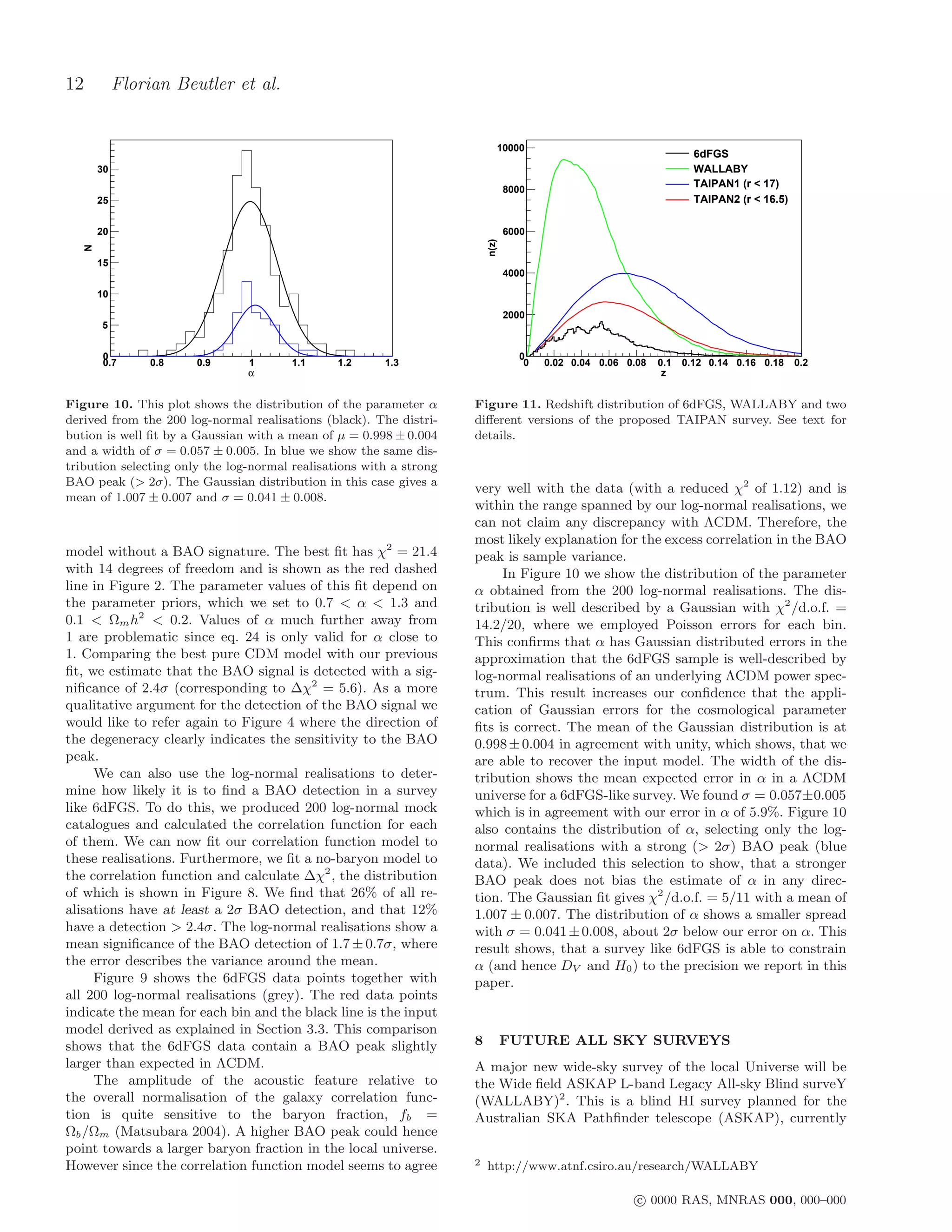
20
10
0
-10
-20
0 20 40 60 80 100 120 140 160 180 200
s [h-1Mpc]
Figure C2. The black line represents the plain correlation func-
tion without redshift space distortions (RSD), ξ(r), obtained by
a Hankel transform of our fiducial ΛCDM power spectrum. The
blue line includes the linear model for redshift space distortions
(linear Kaiser factor) using β = 0.27. The red line uses the same
value of β but includes all correction terms outlined in eq. C1
using the N (φ, θ, s) distribution of the weighted 6dFGS sample
employed in this analysis.
such that
π π/2
N (φ, θ, s) dθdφ = 1. (C5)
0 0
If the angle θ is of order 1 rad, higher order terms become
dominant and eq. C1 is no longer sufficient. Our weighted
sample has only small values of θ, but growing with s (see
figure C1). In our case the correction terms contribute only
mildly at the BAO scale (red line in figure C2). However
these corrections behave like a scale dependent bias and
hence can introduce systematic errors if not modelled cor-
rectly.
c 0000 RAS, MNRAS 000, 000–000