This document discusses the potential for x-ray interferometry and the Maxim Pathfinder mission concept. It describes how an x-ray interferometer could achieve much higher resolution than current x-ray telescopes by using multiple collector spacecraft separated by long distances. The Maxim Pathfinder would demonstrate 100 microarcsecond resolution using two spacecraft separated by 450 km. System modeling tools would be crucial for development and optimization of the interferometer design.

1. Webster Cash
University of Colorado
X-ray
Interferometry

2. Collaborators
• Ann Shipley, Karen Doty, Randy McEntaffer,
& Steve Osterman at CU
• Nick White – Goddard
• Marshall Joy – Marshall
• David Windt and Steve Kahn - Columbia
• Mark Schattenburg - MIT
• Dennis Gallagher – Ball Aerospace

3. X-ray Telescopes
X-ray telescopes are sensitive
to material at millions of degrees.

4. Capella 0.1”

5. Capella 0.01”

6. Capella 0.001”

7. Capella 0.0001”

8. Capella 0.00001”

9. Capella 0.000001”

10. AR Lac
Simulation @ 100μas

11. AGN Accretion Disk
Simulations @ 0.1μas
C. Reynolds, U. Colorado
M. Calvani, U. Padua

12. Need Resolution and Signal
If we are going to do this, we need to support
two basic capabilities:
• Signal
• Resolution

13. X-ray Sources Are Super Bright
Example: Mass Transfer Binary
1037ergs/s from 109cm object
That is ~10,000L from 10-4A = 108 B
where B is the solar brightness in ergs/cm2/s/steradian
Brightness is a conserved quantity and is the measure of visibility
for a resolved object
Note: Optically thin x-ray sources can have
very low brightness and are inappropriate
targets for interferometry.
Same is true in all parts of spectrum!

14. Minimum Resolution

15. Status of X-ray Optics
• Modest Resolution
– 0.5 arcsec telescopes
– 0.5 micron microscopes
• Severe Scatter Problem
– Mid-Frequency Ripple
• Extreme Cost
– Millions of Dollars Each
– Years to Fabricate

16. Classes of X-ray Interferometers
Dispersive
Non-Dispersive
Elements are Crystals or Gratings
Elements are Mirrors Telescopes

17. Achieving High Resolution
Use Interferometry to Bypass Diffraction Limit
Michelson Stellar Interferometer
R=λ/20000D
R in Arcsec
λ in Angstroms
D in Meters

18. Creating Fringes
Requirements
• Path Lengths Nearly Equal
• Plate Scale Matched to Detector
Pixels
• Adequate Stability
• Adequate Pointing
• Diffraction Limited Optics
D d

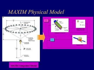
19. δ
sin
B1=
θ
B2 = B1cos(2θ )
[ ( )] δ θ
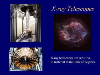
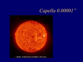
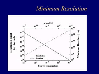
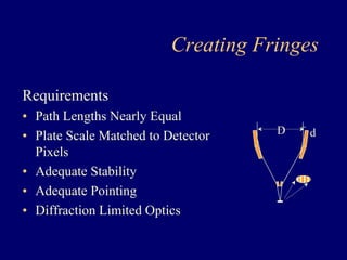
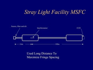
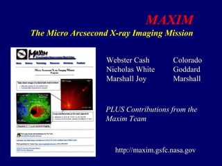
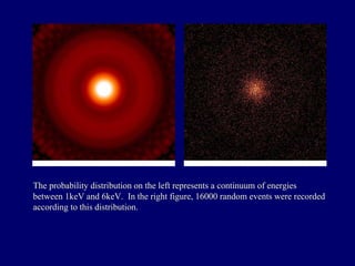
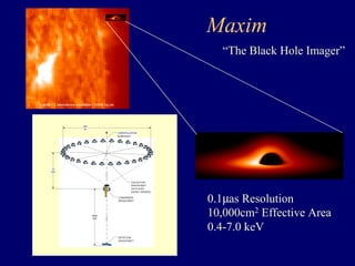
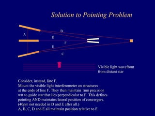
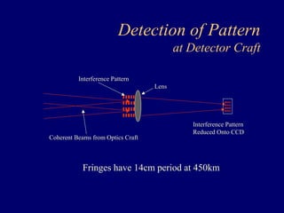
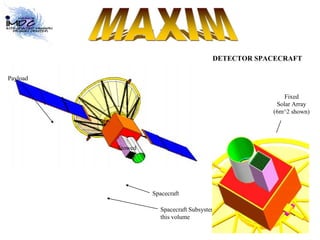
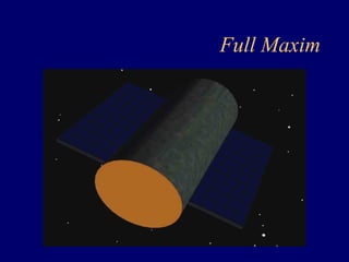
Pathlength Tolerance Analysis at Grazing Incidence
OPD = B1− B2 = 1− cos 2 =
δ θ 2 sin
θ
sin
θ
δ λ
20sin
θ Β2 If OPD to be λ/10 then
( )
λ
θ θ
20sin cos
d Baseline
( )
θ
λ
20sin2
d focal
A1 A2
S1
S2
δ
A1 A2 in Phase Here
C
θ
θ
θ
Β1

20. A Simple X-ray Interferometer
Flats Beams Cross
Detector

21. Wavefront Interference
λ=θs (where s is fringe spacing)
θ=d/L
s = L λ s
d

22. Optics
Each Mirror Was Adjustable
From Outside Vacuum
System was covered by thermal shroud

23. Stray Light Facility MSFC
Source, filter and slit
16m
Interferometer CCD
100m
Used Long Distance To
Maximize Fringe Spacing

24. CCD Image @ 1.25keV
2 Beams Separate 2 Beams Superimposed

25. Fringes at 1.25keV
Profile Across Illuminated Region

26. Test Chamber
at CU
Ten Meter Long Vacuum
Chamber for Testing
Came on-line early May
EUV results good
Upgrade to x-ray next

27. Actual Image at 30.4nm
Image of Slit
Reconstructed from 4 azimuths

28. MAXIM
The Micro Arcsecond X-ray Imaging Mission
Webster Cash Colorado
Nicholas White Goddard
Marshall Joy Marshall
PLUS Contributions from the
Maxim Team
http://maxim.gsfc.nasa.gov

29. Target Class Goal
Maxim:
A Few Science Goals
Resolve the corona of nearby stars: Are other coronal structures like the solar corona?
Resolve the winds of OB stars: What kind of shocks drive the x-ray emission?
Resolve pre-main sequence stars: How does coronal activity interact with disk?
Image of center of Milky Way: Detect and resolve accretion disk?
Detailed images of LMC, SMC, M31: Supernova morphology and star formation in other settings
Image jets, outflows and BLR from AGN: Follow jet structure, search for scattered emission from BLR
Detailed view of starbursts: Resolve supernovae and outflows
Map center of cooling flows in clusters: Resolve star formation regions?
Detailed maps of clusters at high redshift: Cluster evolution, cooling flows
Image Event Horizons in AGNS: Probe Extreme Gravity Limit

30. Flats Held in Phase
Sample Many Frequencies

31. As More Flats Are Used
Pattern Approaches Image
2 4 8
12 16 32

32. On the left is the probability distribution function for two sources in the same
field of view. The central source has an energy half that of the source that is
displaced to the lower left. The image on the right shows 9000 total events for
this system with the lower energy source having twice the intensity of the higher
energy source. Even though the higher energy source is in the first maxima of
the other, the two can still be easily distinguished.

33. Clockwise from upper left: Probability distribution; 100 photons randomly plotted; 9000
photons; and 5000 photons.

34. These figures show the probability distribution for the 6keV portion of the
continuum and the contribution of photons with energies between 5-6keV to
the data simulation.

35. These figures show the probability distribution for the 1keV portion of the
continuum and the contribution of photons with energies between 0-1keV to
the data simulation.

36. The probability distribution on the left represents a continuum of energies
between 1keV and 6keV. In the right figure, 16000 random events were recorded
according to this distribution.

37. Stars
Simulation with Interferometer
Sun with SOHO

38. AGN with Jet
3C273 with Chandra
Simulation with Interferometer

39. Four Difficult Areas
• Fabrication of Interferometer
• Internal Metrology
– Hold Mirrors Flat and In Position
• Formation Flying
– Hold Detector Craft in Position
• Pointing
– Hold Interferometer on Target

40. Maxim
“The Black Hole Imager”
0.1μas Resolution
10,000cm2 Effective Area
0.4-7.0 keV
CONVERGER
SPACECRAFT
DETECTOR
SPACECRAFT
200
M
COLLECTOR
SPACECRAFT
(32 PLACES
EVENLY SPACED)
10
KM
5000
KM
CONSTELLATION
BORESIGHT

41. Maxim Pathfinder
100μas Resolution
100cm2 Effective Area
0.4-2.0keV + 6keV
Two Spacecraft
Formation Flying at
450km Separation

42. 2.5m
10m
Optics Spacecraft
Carries: X-ray Interferometers
Finder X-ray Telescopes
2 Visible Light Interferometers
Laser Ranging System
Size: 2.5x2.5x10m
PitchYaw Stability: 3x10-4 arcsec
PitchYaw Knowledge: 3x10-5 arcsec
Roll Stability: 20 arcsec
Position Stability: -----
Detector Spacecraft
Carries: X-ray Detector Array
Laser Retro Reflectors
Precision Thrusters
Size: 1x1x1m
PitchYaw Stability: 20 arcsec
Roll Stability: 20 arcsec
Lateral Stability: 5mm
Lateral Knowledge: 50 microns
Focal Stability: 10 meters
1m
1m
Separation 450km
Maxim Pathfinder Mission Concept

43. Optics Craft
Prime Interferometer
Wolter Telescope
Pitch Sensor
Yaw Sensor
Front View

44. Solution to Pointing Problem
A
B
C
D
E
F
Visible light wavefront
from distant star
Consider, instead, line F.
Mount the visible light interferometer on structures
at the ends of line F. They then maintain 1nm precision
wrt to guide star that lies perpendicular to F. This defines
pointing AND maintains lateral position of convergers.
(40pm not needed in D and E after all.)
A, B, C, D and E all maintain position relative to F.

45. Detector
• Energy Resolution Necessary for Fringe
Inversion
• CCD is adequate
• To get large field of view use imaging
quantum calorimeter

46. Metrology
Tightest Tolerance is Separation of Entrance Apertures
d = λ/20θ for tenth fringe stability
At 1keV and 2deg, d=1.7nm
At 6keV and 0.5deg, d=1.1nm
Requires active thermal control and internal alignment

47. Laser
Beamsplitter
Laser Beam
Split and Collimated
Collimator
Collimated Beams
Cross at 450km
Optics Craft
450km to
Detector Craft

48. Detection of Pattern
Interference Pattern
Coherent Beams from Optics Craft
Lens
at Detector Craft
Interference Pattern
Reduced Onto CCD
Fringes have 14cm period at 450km

49. Pointing
Need stability and information wrt to the celestial sphere
at level of required resolution.
L2 or Fly-away orbit probably necessary
Baseline design calls for two stellar interferometers.
One each for pitch and yaw
SIM class interferometers more than adequate

50. Delta IV (H) 5m diameter x 19.8m long
Launch Fairing Removed
Detector Spacecraft
(2.2m)
Optics Instruments
(10m)
Optic Spacecraft Systems
(2.2m)
Baffling
LAUNCH
CONFIGURATION
16.4 m
15.5 m
Payload
Spacecraft

51. ORBIT CONFIGURATION
Optic Spacecraft
Detector Spacecraft
Solar Array
(7 m^2, projected area)

52. Stowed
DETECTOR SPACECRAFT
Orbit
Payload
Spacecraft
Spacecraft Subsystems are mounted in
this volume
Fixed
Solar Array
(6m^2 shown)

53. MAXIM Trajectory in Solar Rotating
Coordinates

54. Maxim Pathfinder

55. Maxim Design
CONVERGER
SPACECRAFT
DELAY LINE
DETECTOR
SPACECRAFT
200
M
COLLECTOR
SPACECRAFT
(32 PLACES
EVENLY SPACED)
10
KM
5000
KM
CONSTELLATION
BORESIGHT
Hub Spacecraft
SPACECRAFT
Light from Star
Hub Craft Converger Craft Delay Craft

56. Full Maxim

57. Maxim Limitations
• If primary flats are on separate spacecraft
then they can be flown farther apart.
Resolution increases.
• Limited by visible light aspect from stars
– They’re all resolved at 30nano-arcsec!
• Find non-thermal visible sources
• Use x-ray interferometry for aspect too.
• Solve aspect problem and reach 10-9 arcsec

58. Integrated System Modeling
Ball Aerospace Technologies Corporation
M. Lieber
D. Gallagher
Will lead to single most important tool in development
and definition of x-ray interferometry

59. Integrated End-to-End Modeling Environment
• Integrated modeling seamlessly combines the subsystem models from well
established software tools.
• Allows one to rapidly study parameter interaction of disparate variables from
different disciplines. Integrated models facilitate GUI development - muliti-user
system tool.
• Standard interfaces minimizes errors and miscommunications between disciplines
Control System
Structure
Design Control System
Structure
Design
Optics/Sensor
Design Optics/Sensor
Design
Design
Design
CODE V/
various
NNAASSTTRRAANN SSimimuulinlink/kM/MAATTLLAABB CODE V/
various
STRUCTURE OPTICS/S
ENSOR
DESIGN PARAMETERS
Thermal
Disturbances
Thermal
Disturbances
Mechanical
Disturbances
Mechanical
Disturbances
OOpptitciacla El Errrororsrs
MODELING
TOOLS
TRASYS/
SINDA
MMAATTLLAABB
TRASYS/
SINDA
CCOODDEE V V
ENVIRONMENT
INPUTS
SYSTEM PERFORMANCE
VS.
SCIENCE METRICS
Sensor
Noise MATLAB MATLAB
Sensor
Noise
SYSTEM MODEL
Simulink/MATLAB
CONTROLS

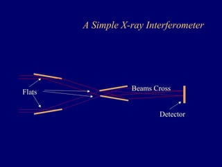
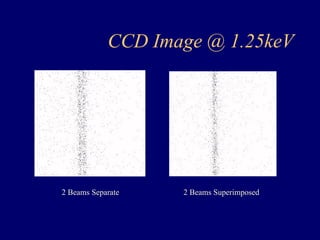
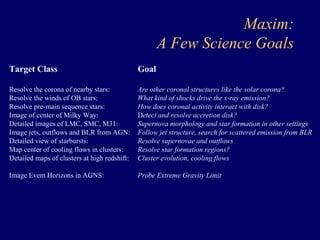
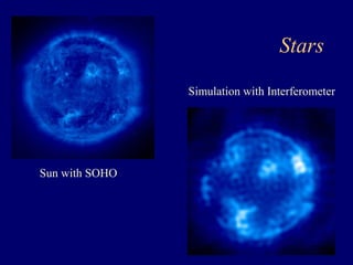
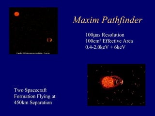
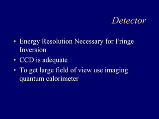
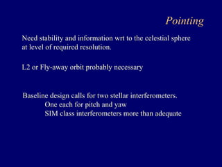
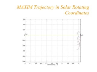
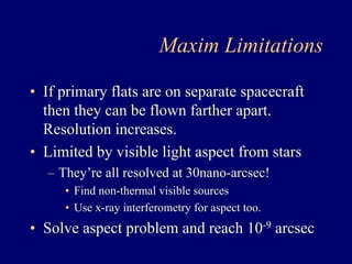
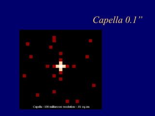
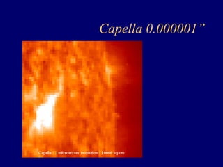
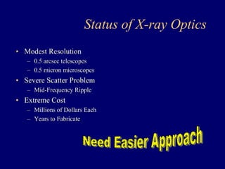
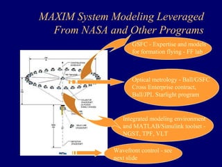
60. Example of MAXIM Pathfinder
Maxim Pathfinder IM
2
Wavefront tilt
sensor models
1
Signal
processing
Telescope mechanism
tip/tilt and
wavefront control
systems
Structural
dynamics
Spacecraft
attitude
control
Optics
model
Image
processing
Imaging sensor
3 models
1
In1
2
sav_psf
Optical subsystem
Sparse To Workspace2
secondary mirror
array
Sparse
primary mirror
array
Optical ray
bundle1
RB offsets
Deform map
Out3
Offsets1
RB offsets
Deform map
Out3
Offsets
Image
plane
[ttt,uuu]
[ttt,uuu2]
u_surf2
u_surf1
1
Out1
Sparse reflective
{a1} mirror1
Sparse reflective
mirror2
Sparse reflective
mirror3
Sparse reflective
mirror4
{b1}
[c1]
[c2]
[c3]
[c4]
1
Ray bundle
{a1} {b1}
[c1]
[c2]
[c3]
[c4]
2
Optics
motion
• Structures, optics,
controls, signal
processing, disturbances

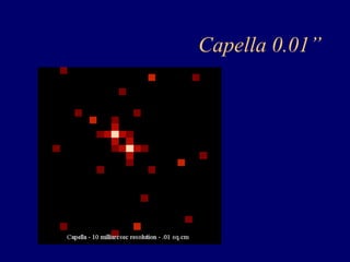
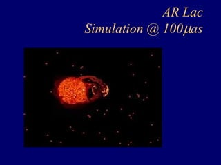
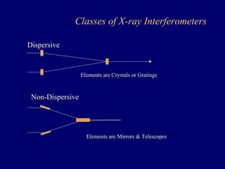
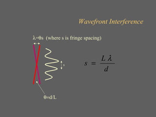
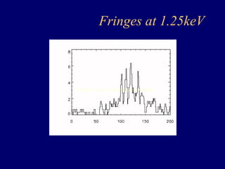
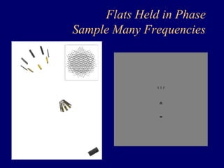
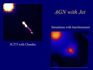
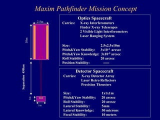
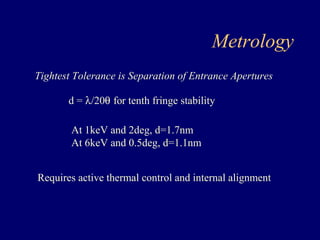
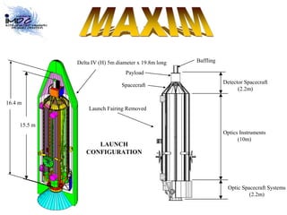
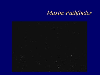
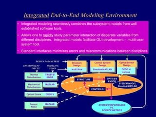
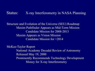
61. Optical Toolbox:
Key Element of Optical Performance Modeling
• Geometric ray trace
• Diffraction analysis (PSF outputs)
• Easy introduction of mirror distortions from thermal or
vibration
• Optics tied to NASTRAN structural model
• Active control modeling of metrology system and active
optics
• Interfaces with imaging and detection modules
sav_psf
Sparse To Workspace2
secondary mirror
array
Sparse
primary mirror
array
Optical ray
bundle1
RB offsets
Deform map
Out3
Offsets1
RB offsets
Deform map
Out3
Offsets
Image
plane
[ttt,uuu]
[ttt,uuu2]
u_surf2
u_surf1
See
next
slide

62. MAXIM Pathfinder PSFs with Different
Number of Optical Elements
2 segments
4 segments
32 segments
PSF Image Log image

63. MAXIM Physical Model
MAXIM Integrated Model
Celestrial
objects
Converger and
Delay Line S/C
Detector S/C
Collectors Hub S/C
Command
and Control

64. MAXIM System Modeling Leveraged
From NASA and Other Programs
GSFC - Expertise and models
for formation flying - FF lab
Optical metrology - Ball/GSFC
Cross Enterprise contract,
Ball/JPL Starlight program
Integrated modeling environment
and MATLAB/Simulink toolset -
NGST, TPF, VLT
Wavefront control - see
next slide

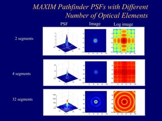
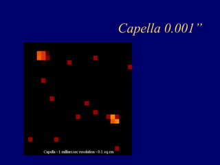
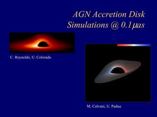
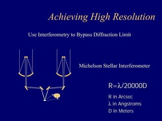
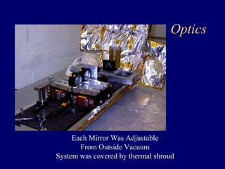
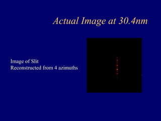
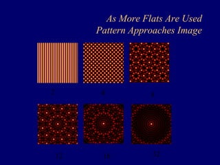
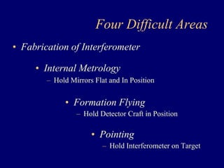
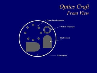
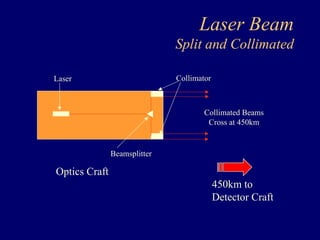
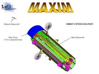
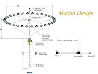
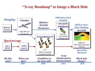
65. Example Wavefront Control Modeling -
Initial Phase Map of NGST
• Wavefront control tools from NGST program and extensive
work on phase retrieval by JPL
10 20 30 40 50 60
10
20
30
40
50
60
10 20 30 40 50 60
10
20
30
40
50
60
Random errors for 36 segments
• RMS random = primary
segments [ 1e-4 1e-4 4e-5 1e-5 1e-4 0]
[ x-decenter y-decenter piston tip tilt clocking]
• Secondary =
offsets
10x 10-4
0 2 4 6 8
-2
-4 1 2 3 4 5 6
[ 1e-3 5e-4 1.5e-5 -3e-5 8e-4
0]
[ x-decenter y-decenter piston tip tilt clocking]
x-decenter
y-decenter
piston
tip
tilt

66. Status: X-ray Interferometry in NASA Planning
Structure and Evolution of the Universe (SEU) Roadmap
Maxim Pathfinder Appears as Mid-Term Mission
Candidate Mission for 2008-2013
Maxim Appears as Vision Mission
Candidate Mission for 2014
McKee-Taylor Report
National Academy Decadal Review of Astronomy
Released May 19, 2000
Prominently Recommends Technology Development
Money for X-ray Interferometry

67. “X-ray Roadmap” to Image a Black Hole
Imaging
Spectroscopy
Do they
exist?
X-ray
Interferometry
Demonstration
Million times
finer imaging
Black hole
Imager!
Where are
they?
Optimize
MAXIM
Parameters
Conditions in
the inner disk
2000 2008 2014 2020
ROSAT
Einstein
ASCA
RXTE
1000 times finer
imaging
MAXIM
Pathfinder
100 cm2
2 m baseline
100 μarc sec
MAXIM
1000 cm2
100-1000 m baseline
100 nas
Chandra
100-1000 cm2
0.5 arc sec
XMM
Astro-E
Constellation-X
3 m2
Indirect imaging
via spectroscopy
Spectrally
Resolved

68. Plan
• Technology Development
– Start with NIAC and SRT Funding
– Mission Specific Funding
• Maxim Pathfinder
– New Start 2008
– Develop Test Technology for Maxim
• MAXIM
– Five Years after Pathfinder

69. The Black Hole
Disney, 1979
We have already found this black hole and will have these
pictures before 2020.