This study focuses on imaging the host galaxy of the quasar 3C 273 using coronagraphic techniques with the Hubble Space Telescope. By removing overwhelming quasar light through reference star observations, the research reveals new structures in the host galaxy, including a core jet and smaller-scale blobs, suggesting possible satellite galaxies. The findings validate the use of coronagraphs to gain insights into quasar hosts and their environments in high-resolution visible light.

1. Astronomy & Astrophysics manuscript no. ms ©ESO 2024
16th
February, 2024
Letter to the Editor
3C 273 Host Galaxy with Hubble Space Telescope Coronagraphy⋆
Bin B. Ren (任彬) iD ⋆⋆1, 2, 3, 4, 5, Kevin Fogarty iD 6, 3, John H. Debes iD 7, Eileen T. Meyer iD 8, Youbin Mo9⋆⋆⋆, Dimitri
Mawet iD 3, 10, Marshall D. Perrin iD 7, Patrick M. Ogle7, and Johannes Sahlmann iD 11
1
Université Côte d’Azur, Observatoire de la Côte d’Azur, CNRS, Laboratoire Lagrange, Bd de l’Observatoire, CS 34229, F-06304
Nice cedex 4, France; bin.ren@oca.eu
2
Université Grenoble Alpes, CNRS, Institut de Planétologie et d’Astrophysique (IPAG), F-38000 Grenoble, France
3
Department of Astronomy, California Institute of Technology, MC 249-17, 1200 E California Blvd, Pasadena, CA 91125, USA
4
Department of Physics and Astronomy, The Johns Hopkins University, 3701 San Martin Drive, Baltimore, MD 21218, USA
5
Department of Applied Mathematics and Statistics, The Johns Hopkins University, 3400 N Charles St, Baltimore, MD 21218,
USA
6
NASA Ames Research Center, Moffett Field, CA 94035, USA; kevin.w.fogarty@nasa.gov
7
Space Telescope Science Institute (STScI), 3700 San Martin Drive, Baltimore, MD 21218, USA
8
Department of Physics, University of Maryland, Baltimore County, 1000 Hilltop Circle, Baltimore, MD 21250, USA
9
Department of Physics, University of California, San Diego, CA 92093, USA
10
Jet Propulsion Laboratory, California Institute of Technology, 4800 Oak Grove Drive, Pasadena, CA 91109, USA
11
RHEA Group for the European Space Agency (ESA), European Space Astronomy Centre (ESAC), Camino Bajo del Castillo s/n,
E-28692 Villanueva de la Cañada, Madrid, Spain
Received 12 October 2023 / Revised 14 February 2024 / Accepted 14 February 2024
ABSTRACT
The close-in regions of bright quasars’ host galaxies have been difficult to image due to the overwhelming light from the quasars. With
coronagraphic observations in visible light using the Space Telescope Imaging Spectrograph (STIS) on the Hubble Space Telescope,
we removed 3C 273 quasar light using color-matching reference stars. The observations revealed the host galaxy from 60′′
to 0′′
.2
with nearly full angular coverage. Isophote modeling revealed a new core jet, a core blob, and multiple smaller-scale blobs within
2′′
.5. The blobs could potentially be satellite galaxies or infalling materials towards the central quasar. Using archival STIS data, we
constrained the apparent motion of its large scale jets over a 22 yr timeline. By resolving the 3C 273 host galaxy with STIS, our study
validates the coronagraph usage on extragalactic sources in obtaining new insights into the central ∼kpc regions of quasar hosts.
Key words. (Galaxies:) quasars: individual: 3C 273 – Methods: observational – Instrumentation: high angular resolution
1. Introduction
Quasars are unique laboratories for the extreme physics govern-
ing active galactic nuclei (AGN) accretion and feedback, and are
important drivers for galaxy evolution and enrichment (e.g., Si-
jacki et al. 2007; McNamara & Nulsen 2012; Moustakas et al.
2019). However, since the central source in a quasar can have
a visual luminosity comparable to the entire host galaxy within
which it resides, the point spread function (PSF) of a quasar’s
central source – when seen with a telescope with finite mirror
size – often dominates the light at inner ∼kpc scales. Many fea-
tures of quasars’ circumnuclear regions (e.g., Ramos Almeida &
Ricci 2017), such as inflows, dusty tori, winds, and jets, have
visual and infrared components that are overwhelmed as a re-
sult (e.g. Ford et al. 1994, 2014). Moreover, the dynamics and
morphology of the host galaxy close-in to the nuclear region are
likewise “swamped out” in visible and near-infrared (NIR) ob-
servations. While advances in radio interferometry have allowed
us to glimpse the event horizons of two supermassive black holes
⋆
FITS images for Figs. 1–2 are only available at the CDS via
anonymous ftp to cdsarc.cds.unistra.fr (130.79.128.5) or via
https://cdsarc.cds.unistra.fr/viz-bin/cat/J/A+A/
⋆⋆
Marie Skłodowska-Curie Fellow
⋆⋆⋆
Now at Google.
at ∼0.1 mas scale and their surrounding environments (i.e., M87:
Event Horizon Telescope Collaboration et al. 2019, Sagittar-
ius A*: Event Horizon Telescope Collaboration et al. 2022; Lu
et al. 2023), many processes critical to feeding and feedback in
extremely luminous quasars will only be understood once we
obtain high-contrast, high-resolution imaging in the visible and
NIR (e.g., Martel et al. 2003; Gratadour et al. 2015; Brandl et al.
2008; Moustakas et al. 2019; Rouan et al. 2019; Grosset et al.
2021; Ding et al. 2023).
To study quasar hosts, infrared and radio interferometry are
capable of imaging the inner several parsecs of the circumnu-
clear region, and can therefore look at the broad line region, in-
ner radius of the torus, and jets on this scale (e.g. Kishimoto et al.
2011; Lister et al. 2013; Gravity Collaboration et al. 2018). How-
ever, circumnuclear disk, infalling material, and jet activity in
the narrow-line region are best observed at an intermediate scale
in the further out regions. To study these regions, observations
of naturally dust-obscured quasars (“natural coronagraphs”; e.g.,
Jaffe et al. 1993; van der Marel & van den Bosch 1998) only
preferentially sample these structures in disk-like hosts or during
epochs of peak dust production early-on in mergers, giving an in-
complete picture of quasar evolution (Urrutia et al. 2008; Schaw-
inski et al. 2012; Del Moro et al. 2017). The Space Telescope
Imaging Spectrograph (STIS) coronagraph onboard the Hubble
Article number, page 1 of 13
arXiv:2402.09505v1
[astro-ph.GA]
14
Feb
2024

2. A&A proofs: manuscript no. ms
Space Telescope (HST), however, can fill the gap at >0.5 kpc to
∼kpc scales and larger to study the morphology of host galaxies.
Visual imaging of the sub-kpc structures of the dust, jet, and host
galaxies of quasars with STIS coronagraph provides a unique op-
portunity to complement ground- and space-based infrared high-
contrast imaging with Keck and JWST.
The prototypical quasar 3C 273 was first identified based on
its redshift of 0.158 by Schmidt (1963). With the central quasar
dominating the signals across visible to radio wavelengths and
thus overwhelming the host galaxy, the study of the latter makes
it necessary to first properly remove the quasar light. In visi-
ble wavelengths, Martel et al. (2003) placed the 3C 273 be-
hind a coronagraph using HST/ACS, removed the quasar light
using reference star images, and revealed the host galaxy in
visible light exterior to an angular radius of ∼1′′
.5. With non-
coronagraphic imaging after empirical PSF removal, these non-
asymmetric signals persist after host galaxy modeling (Zhang
et al. 2019, Figure 10 therein). In (sub)-millimeter observa-
tions Komugi et al. (2022) subtracted point source models us-
ing ALMA, and revealed the surroundings where the millime-
ter continuum emission colocates with the extended emission
line region in [O III] observed with VLT/MUSE in Husemann
et al. (2019). These efforts unveiled complex structure for the
3C 273 host from multiple aspects, calling for dedicated imaging
that would better reveal and characterize the 3C 273 host with
available state-of-the-art instruments. Here we report our coro-
nagraphic high-contrast imaging observations using HST/STIS,
where we reached an inner working angle (IWA) of ∼0′′
.2 in vis-
ible light to reveal the 3C 273 host galaxy.
2. Observation and Data Reduction
The HST/STIS coronagraph offers broadband imaging in visi-
ble through NIR light (0.2 µm – 1.15 µm; Medallon & Welty
2023). Its narrowest occulter BAR5 can image the surroundings
of bright sources exterior to ∼0′′
.2 from the center (Schneider
et al. 2017; Debes et al. 2019). To reveal the surroundings of
bright central sources using STIS, a careful selection of refer-
ence stars is needed to avoid color mismatch given its broadband
(Debes et al. 2019), otherwise a non-matching PSF can induce
spurious signals (Ren et al. 2017, Figure 8 therein). A reference
star should be of similar color, magnitude, and in close proxim-
ity of a science target to maximize the success in coronagraphic
imaging (Debes et al. 2019). To explore the inner regions of the
3C 273 host galaxy down to ∼0′′
.2, or ∼0.5 kpc,1
we observed
it with two reference stars using HST/STIS in HST GO-16715
(PI: B. Ren). The two reference stars serve as the empirical PSF
templates to remove the 3C 273 quasar light.
2.1. PSF reference star selection
On the lower Earth orbit, HST is affected by instrumental effects
such as breathing caused by changes in the Solar angle, radi-
ation, and Earth’s shadow. These effects on STIS observations
could be empirically captured and removed when well-chosen
PSF stars are close in angle to the science target. To effectively
remove the PSF from the central source, Debes et al. (2019) rec-
ommended close match in magnitude and color in the B and
V band. With the high-sensitivity space-based measurements in
visible light from the Gaia mission (DR3: Gaia Collaboration
et al. 2023), Walker et al. (2021) showed that magnitude and
1
0′′
.1 = 0.27 kpc for 3C 273 in ΛCDM cosmology with Ωm = 0.27,
ΩΛ = 0.73, and H0 = 71km s−1
Mpc−1
.
color match in Gaia filters may also provide reasonably good
PSFs for STIS observations.
Using Gaia DR3, we selected two reference stars –
TYC 287-284-1 (hereafter “PSF1”) and TYC 292-743-1 (here-
after “PSF2”) – to serve as the PSF templates for 3C 273
(hereafter “science target”), see Appendix A. For 3C 273, its
Gaia DR3 magnitude G = 12.84, color Bp − Rp = 0.494 and
G − Rp = 0.348. Within 4◦
.7 from 3C 273, the chosen PSF1
has Gaia DR3 magnitude G = 12.77, color Bp − Rp = 0.515
and G − Rp = 0.327. Within 2◦
.7 from 3C 273, the chosen
PSF2 has magnitude G = 11.488, color Bp − Rp = 0.536 and
G − Rp = 0.340. By choosing two PSF reference stars with such
faintness that do not have existing infrared excess measurements,
with infrared excess being indicative of circumstellar disks (e.g.,
Cotten & Song 2016), we can reduce the probability that a refer-
ence star might host a circumstellar disk that negatively impacts
the PSF removal for 3C 273. In addition, this strategy reduces
the possibility that background objects, which are beyond the de-
tection limits of exiting instruments, negatively impact the PSF
removal of 3C 273.
2.2. Observation
Coronagraphic imaging with HST/STIS relies on the blockage
of light in central regions using its physical occulters. In STIS,
BAR5 and WedgeA0.6 are two nearly perpendicular occult-
ing locations that offer IWAs of ∼0′′
.2 and ∼0′′
.3, respectively
(Medallon & Welty 2023). To enable a full angular coverage
of extended structures, however, the two locations are near to
the edges of the field of view of STIS, making it unrealistic to
roll the telescope ∼90◦
to achieve a nearly 360◦
coverage given
the scheduling limits of HST using four consecutive orbits (e.g.,
Figure 3 of Debes et al. 2019),2
see Appendix A. Therefore, we
scheduled two sets of observations in GO-16715, and each set
is composed of 4 contiguous “back-to-back” HST orbits, see Ta-
ble A.1 for the observation log. By observing 3C 273 at two
different epochs spanning ∼2 months in HST Cycle 29, the rel-
ative roll is 84◦
.032 between the central visits of the two epochs
to approach a full angular coverage.
In GO-16715, we observed only one object in an orbital visit,
with a sequence of “target-target-PSF-target” in a 4-orbit obser-
vation set. This ensures that the telescope thermal distribution is
stabilized when a PSF star is observed. The observations were
in CCD Gain = 4 mode to permit high dynamic range imaging
(e.g., Debes et al. 2019). For the 3 orbits on the target, we rolled
the telescope by either ±15◦
(UT 2022-01-08) or ±5◦
(UT 2022-
03-26)3
to approach a ∼360◦
angular coverage for it, see Fig. B.1
for the coverage map of 3C 273.
Within one science target orbit, we observed 3C 273 using
both the BAR5 and the WedgeA0.6 occulting location with 3
readouts each. With three readouts each being a 315 s exposure
at an occulting location, the STIS flat-fielded files can identify
cosmic rays for random noise removal. There are a total of 36
readouts from 6 orbits. For the reference stars, on the one hand,
the Gaia DR3 G magnitude of PSF1 is similar as that of the sci-
ence target, with PSF1 being 0.07 mag brighter. The observation
strategy of PSF1 is identical to the target: to reach similar detec-
2
For observation planning, see Phase 2 of Astronomer’s Proposal Tool
(APT) for actual roll ranges for given observation times.
3
Roll angle of ±5◦
due to updated scheduling constraints with the HST
guide star catalog then. When permitted, ±22◦
.5 rolls can maximize an-
gular coverage by avoiding HST diffraction spikes that are along the
(off)-diagonal directions in STIS images.
Article number, page 2 of 13

3. Ren et al.: 3C 273 with HST/STIS Coronagraphy
-2000
-1000
000
1000
2000
R.A.
-2000
-1000
000
1000
2000
Decl.
+
E
N
10 kpc
10 1
100
101
102
[×10
20
erg
s
1
cm
2
Å
1
]
Fig. 1. 3C 273 host galaxy and surroundings in visible light seen with the HST/STIS coronagraph. The surface brightness is in log scale.
(The data used to create this figure are available.)
tor counts, each readout of PSF1 is 294 s. There are 6 readouts
in total for PSF1. On the other hand, the Gaia DR3 G magnitude
of PSF2 is 1.352 mag brighter than that of the science target. To
reach similar detector counts as 3C 273, each readout of PSF2
is 125 s. Given the available time in one HST orbit, the rela-
tively shorter readout time permit the dithering of the telescope:
the on-sky step is 0.25 STIS pixel to reduce the impact from
the non-repeatability of HST pointing on STIS results (e.g., Ren
et al. 2017; Debes et al. 2019). At each occulting location, we
dithered the telescope twice with each dithering location having
two 125 s readouts, totaling 6 readouts per occulting location.
There are a total of 12 readouts for PSF2.
2.3. Data reduction
2.3.1. Pre-processing
In long readouts (315 s for the target), the observation data
quality with STIS may be compromised due to different noise
sources (e.g., cosmic ray, shot noise, charge transfer ineffi-
ciency: CTI). To address this in data reduction, we first used the
stis_cti package4
that applies the Anderson & Bedin (2010)
correction to remove CTI effects for STIS CCD.5
We then used
the data quality map in the CTI-corrected flat-fielded files, and
followed Ren et al. (2017) to perform a median bad pixel re-
placement for the data that have been marked as a bad pixel
(e.g., pixels with dark rate more than 5σ the median dark level,
bad pixel in reference file, and pixels identified in cosmic ray
rejection) around its 3×3-pixel neighbors. To correct for the ge-
4
https://pythonhosted.org/stis_cti/
5
See https://github.com/spacetelescope/STIS-Notebooks
for a usage example of stis_cti under DrizzlePac.
Article number, page 3 of 13

4. A&A proofs: manuscript no. ms
ometric distortion in 2-dimensional STIS CCD images (Hodge
et al. 1998), we then rectified the CTI-corrected images using the
x2d function from stistools.6
In STIS coronagraphic imaging, the central star is blocked
by the STIS occulters, we thus used the two diffraction spikes to
align the images (e.g., Schneider et al. 2014; Ren et al. 2017).
We used the “X marks the spot” method (e.g., Schneider et al.
2014): we first fit Gaussian profiles to each column or row of the
observation to identify the peak of the diffraction spikes, then fit
lines and obtain the intersection point as the location of the star.
In this way, we can obtain both the locations and their associated
uncertainties from the observed data.
2.3.2. Post-processing: PSF removal
For each target image, we minimized the standard deviation for
the regions containing diffraction spikes after PSF subtraction
to obtain a residual image. Specifically, we used the algorithmic
mask from Debes et al. (2017) to identify the regions that are
blocked by the STIS occulters in the observations. At each oc-
culting location, we scaled the median of all the PSF readouts,
and subtracted it from the target readouts to inspect the residual
images. We derotated each residual map to north-up and east-left
using its corresponding ORIENTAT header, and used the element-
wise median of all 36 residual maps (18 from each occulting lo-
cation) as the final image for 3C 273 host galaxy. We multiplied
the final image in units of counts s−1
pixel−1
by PHOTFLAM =
4.22 × 10−19
, which is the inverse sensitivity parameter recorded
in the FITS file headers, to obtain the calibrated final image in
units of erg s−1
cm−2
Å−1
, see Fig. 1. We also calculated the stan-
dard deviation for the regions that do not host signals in the final
image to obtain the signal-to-noise map, see Fig. B.3.
To inspect the PSF removal quality dependence on differ-
ent PSF references, we have experimented using a single PSF
star for all the images, and we did observe a decrease in signal-
to-noise from combining the two PSF stars. In fact, in the ob-
servations for PSF1, we identified at least two faint background
sources within the STIS field of view (e.g., Fig. A.2). Neverthe-
less, this was anticipated in our observation planning, and we
minimized such risks by using multiple PSF stars in Table A.1.
3. Results
3.1. 3C 273 host
3.1.1. Isophote fitting
We present in Fig. 2 the host galaxy within 5′′
from the quasar.
At the largest spatial scale in Fig. 1, we confirm the existence
of two components – the outer component (OC) and the inner
component (IC) – as previously identified in isophotic contours
in Martel et al. (2003) with HST/ACS. The OC is more extended
on the north-east side than the IC in STIS wavelengths, with both
centers offset from the central quasar, as has been reported in
Martel et al. (2003). With STIS coronagraphy in Fig. 2, we con-
firm the existence of the E1, jet component (JC), and inner jet
(IJ) components identified in Martel et al. (2003).
To reveal small scale structures, we performed isophote mod-
eling to enhance the visibility of structures of smaller spatial
scale. We used the isophote package from photuils (Bradley
et al. 2023), which implemented the Jedrzejewski (1987) method
to iteratively fit elliptical isophotes to the 3C 273 host image. We
6
https://stistools.readthedocs.io/en/latest/x2d.html
present the isophote model in Fig. 2(b) and the model-removed
residuals in Fig. 2(c), where we annotated the structures. To
better reveal these structures, we reperformed isophote fitting
while excluding them to reduce fitting bias, see the final isophote
model and residuals in Fig. 2.
3.1.2. New close-in host structures
We identify a core blob (CB) component at ∼1′′
to the west of
the quasar in Fig. 2(c). We also identify a core jet (CJ) com-
ponent along the direction of the large scale jet. We addition-
ally detect small-scale blobs spanning from 2′′
to 4′′
from the
quasar. These blobs are marked with dotted circles in Fig. 2.
We also detected a more symmetric core component (CC) for
the host galaxy of 3C 273 within ≈1′′
in Fig. 2(a). The sur-
face brightness7
is (5 ± 2) × 10−20
erg s−1
cm−2
Å−1
for CB,
(14 ± 5) × 10−20
erg s−1
cm−2
Å−1
for CC, and (3 ± 2) ×
10−20
erg s−1
cm−2
Å−1
for CJ. In comparison, the background
is (1.3 ± 1.3) × 10−22
erg s−1
cm−2
Å−1
, which is two orders of
magnitude fainter than these new close-in structures. We present
the measurements in Table B.1.
We mark the credible new structures in Fig. 2(c). First, the
CB component is not a random or color-mismatch residual, in
the sense that it does not have a radially shaped elongation that
suggests color mismatch or telescope breathing (e.g., Schnei-
der et al. 2014), and that its globular morphology does not re-
semble the spurious residuals in the existing STIS data archive
for circumstellar structures in Ren et al. (2017). Second, the CJ
component is not only along the direction for the jet, but also
of elliptical shape in the isophote model in Fig. 2(b). Third,
the blobs (i.e., b1, b2, b3) are not risen from random noise and
they are ∼4σ above their surrounding host galaxy (blob sur-
face brightness: ∼4 × 10−21
erg s−1
cm−2
Å−1
): they persist in
the individual reduction results from different telescope rolls
in Fig. B.4, and they are not behind diffraction spikes regions
where random noise may manifest positive residuals. By fitting
the surface brightness of CC with a bivariate normal distribution
while ignoring these small-scale structures, we obtain a semi-
major axis of aCC = 0′′
.578 ± 0′′
.005 and a semi-minor axis of
bCC = 0′′
.477 ± 0′′
.004, and a position angle of 56◦
.2 ± 1◦
.5 for the
major axis. The fitted center is located at ∆R.A. = 0′′
.031±0′′
.004
and ∆Decl. = −0′′
.024±0′′
.003, or 0′′
.039±0′′
.004 from the quasar,
which is less offset from the quasar than IC and OC (0′′
.65–1′′
.40;
Martel et al. 2003). The ellipticity is ηCC = (aCC − bCC)/aCC =
0.175 ± 0.010, which is smaller than the η ≳ 0.3 measurements
in further out regions (Martel et al. 2003, Fig. 4 therein), sug-
gesting that the host galaxy is more symmetric when it is closer
to the quasar.
We detected evidence of extended filamentary structures to
the Northeast, East and West of the galactic nucleus. These struc-
tures are visible in the residuals image (filament surface bright-
ness: ∼2 × 10−21
erg s−1
cm−2
Å−1
) in Fig. 2(c)(d), obtained
after computing and subtracting an elliptical isophote model of
the underlying early-type galaxy. Candidate filaments extending
∼5–10 kpc to the Northeast are reminiscent of the emission line
nebulae seen in e.g. the brightest cluster galaxy in the Phoenix
cluster (McDonald et al. 2018) and believed to be multiphase gas
that condenses out of the circumgalactic medium and fuels fur-
ther AGN feedback (Gaspari et al. 2015, 2018). Structures seen
to the East several kpc from the galactic nucleus and several kpc
to the West are also potentially consistent with this scenario, al-
7
The uncertainties in this Letter are 1σ unless otherwise specified.
Article number, page 4 of 13

5. Ren et al.: 3C 273 with HST/STIS Coronagraphy
R.A.
-400
-200
000
200
400
Decl.
+
E1
IJ
CC
5 kpc
+
-400
-200
000
200
400
R.A.
-400
-200
000
200
400
Decl.
+
JC
CB
E1
IJ
CJ
b1
b2
b3
-400
-200
000
200
400
R.A.
-400
-200
000
200
400
Decl.
+
filament
10 1
100
101
102
[×10
20
erg
s
1
cm
2
Å
1
]
0.6
0.4
0.2
0.0
0.2
0.4
0.6
[×10
20
erg
s
1
cm
2
Å
1
]
Fig. 2. Host galaxy of 3C 273 within 5′′
. (a) contains original data. (b) is the isophote model. (c) and (d) are isophote-removed data. We have
newly identified a symmetric core component (CC) within ∼1′′
(marked with dash dotted circle), a core blob (CB) component at ∼1′′
to the west
of the quasar, a core jet (CJ) component, three smaller scale blobs (marked with dotted circles) at ∼4σ levels in comparison with their surrounding
host galaxy, and filamentary structures at ∼3σ levels. We recover the Martel et al. (2003) findings including jet component (JC), inner jet (IJ), and
E1 component. Note: we masked out a PSF feature (e.g., Grady et al. 2003) in (c) and (d) a shaded ellipse to the east of the center.
(The data used to create this figure are available.)
though either deeper or (ideally) spectroscopic follow-up obser-
vations will be necessary to characterize these structures. Further
multi-band photometric or spectroscopic follow-up observations
with JWST will characterize these structures and determine the
role they play in the lifecycle of AGN feedback in 3C 273.
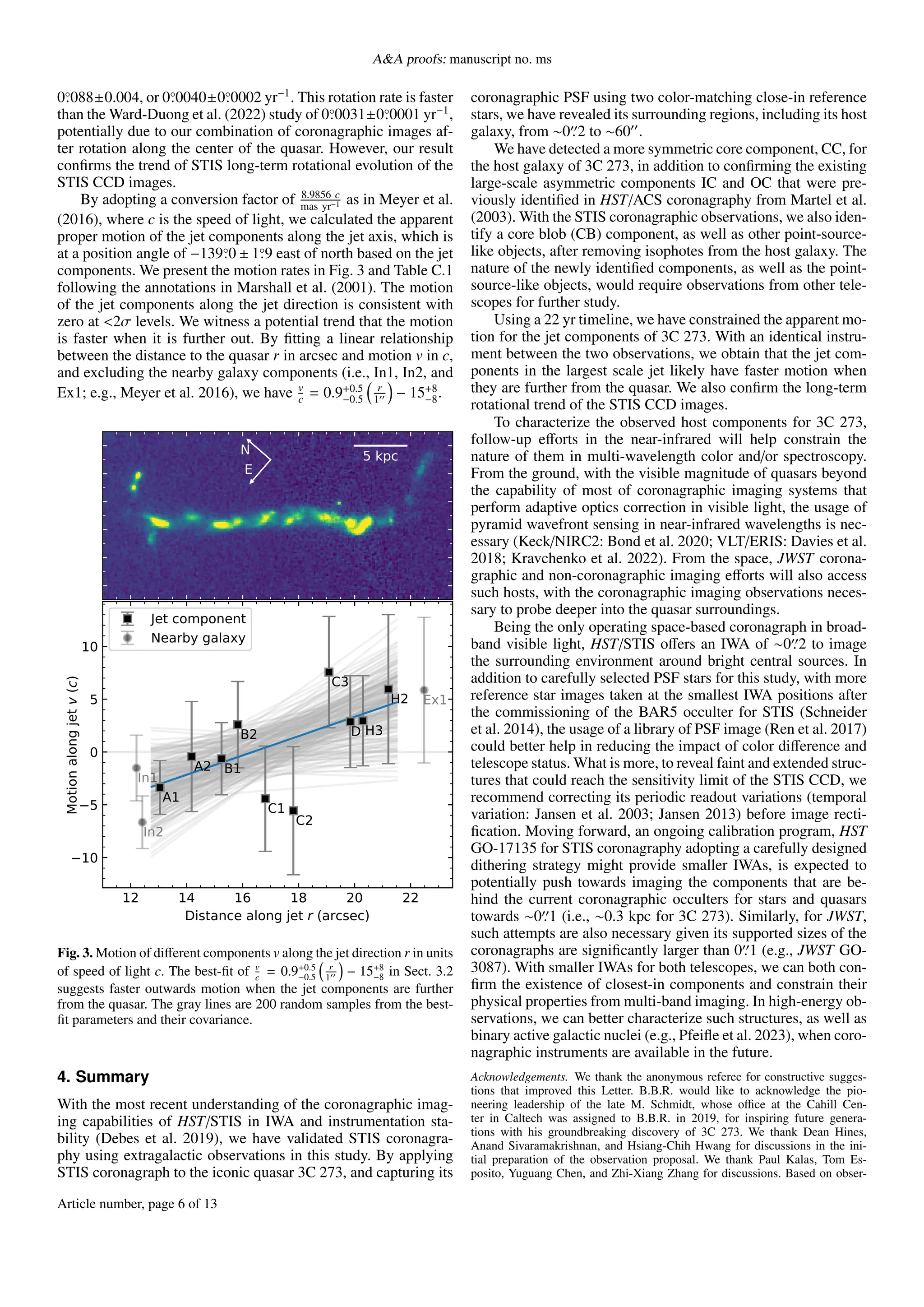
3.2. Jet motion
3C 273 has been imaged with STIS, with the unocculted 50CCD
imaging configuration, on 2000 April 3 in HST GO-8233 (PI:
S. Baum). We do not remove the PSF for this observation us-
ing the coronagraphic archive from Ren et al. (2017), since un-
occulted PSFs do not resemble the coronagraphic ones (Grady
et al. 2003). Nevertheless, the jet is visible in both the 2006 and
our 2022 observations, which establish a 7950–8027 day separa-
tion, or 22 year, for apparent motion measurement.
We aligned the rectified non-coronagraphic observations of
3C 273 with STIS using the “X marks the spot” method. In com-
parison with the coronagraphic observations, there are no data
quality extensions in the flat-fielded files in HST GO-8233, we
thus remove the cosmic ray noises using the Astro-SCRAPPY
code (McCully et al. 2018) that implements the van Dokkum
(2001) approach in astropy (Astropy Collaboration et al.
2013). In comparison with Meyer et al. (2016) where two HST
instruments (WFPC2/PC and ACS/WFC) were used to obtain jet
motion, our study with an identical instrument permits motion
measurements with less offsets from different instruments.
To measure the jet motion between the two epochs using two
images with different quality, we adopted the concept of dummy
variables to simultaneously fit elliptical morphology and offset.
Specifically, for one jet component, we fit identical bivariate nor-
mal distribution to its data in two epochs while allowing for
translation and rotation, see Appendix C for the details.
We also applied the same procedure to measure the offset
for background sources to correct for motion biases due to dif-
ferent observations. The field rotation between the two epochs is
Article number, page 5 of 13

6. A&A proofs: manuscript no. ms
0◦
.088±0.004, or 0◦
.0040±0◦
.0002 yr−1
. This rotation rate is faster
than the Ward-Duong et al. (2022) study of 0◦
.0031±0◦
.0001 yr−1
,
potentially due to our combination of coronagraphic images af-
ter rotation along the center of the quasar. However, our result
confirms the trend of STIS long-term rotational evolution of the
STIS CCD images.
By adopting a conversion factor of 8.9856 c
mas yr−1 as in Meyer et al.
(2016), where c is the speed of light, we calculated the apparent
proper motion of the jet components along the jet axis, which is
at a position angle of −139◦
.0 ± 1◦
.9 east of north based on the jet
components. We present the motion rates in Fig. 3 and Table C.1
following the annotations in Marshall et al. (2001). The motion
of the jet components along the jet direction is consistent with
zero at <2σ levels. We witness a potential trend that the motion
is faster when it is further out. By fitting a linear relationship
between the distance to the quasar r in arcsec and motion v in c,
and excluding the nearby galaxy components (i.e., In1, In2, and
Ex1; e.g., Meyer et al. 2016), we have v
c = 0.9+0.5
−0.5
r
1′′
− 15+8
−8.
5 kpc
N
E
12 14 16 18 20 22
Distance along jet r (arcsec)
10
5
0
5
10
Motion
along
jet
v
(c)
H2
H3
D
C3
C2
C1
B2
B1
A2
A1
Ex1
In2
In1
Jet component
Nearby galaxy
Fig. 3. Motion of different components v along the jet direction r in units
of speed of light c. The best-fit of v
c
= 0.9+0.5
−0.5
r
1′′
− 15+8
−8 in Sect. 3.2
suggests faster outwards motion when the jet components are further
from the quasar. The gray lines are 200 random samples from the best-
fit parameters and their covariance.
4. Summary
With the most recent understanding of the coronagraphic imag-
ing capabilities of HST/STIS in IWA and instrumentation sta-
bility (Debes et al. 2019), we have validated STIS coronagra-
phy using extragalactic observations in this study. By applying
STIS coronagraph to the iconic quasar 3C 273, and capturing its
coronagraphic PSF using two color-matching close-in reference
stars, we have revealed its surrounding regions, including its host
galaxy, from ∼0′′
.2 to ∼60′′
.
We have detected a more symmetric core component, CC, for
the host galaxy of 3C 273, in addition to confirming the existing
large-scale asymmetric components IC and OC that were pre-
viously identified in HST/ACS coronagraphy from Martel et al.
(2003). With the STIS coronagraphic observations, we also iden-
tify a core blob (CB) component, as well as other point-source-
like objects, after removing isophotes from the host galaxy. The
nature of the newly identified components, as well as the point-
source-like objects, would require observations from other tele-
scopes for further study.
Using a 22 yr timeline, we have constrained the apparent mo-
tion for the jet components of 3C 273. With an identical instru-
ment between the two observations, we obtain that the jet com-
ponents in the largest scale jet likely have faster motion when
they are further from the quasar. We also confirm the long-term
rotational trend of the STIS CCD images.
To characterize the observed host components for 3C 273,
follow-up efforts in the near-infrared will help constrain the
nature of them in multi-wavelength color and/or spectroscopy.
From the ground, with the visible magnitude of quasars beyond
the capability of most of coronagraphic imaging systems that
perform adaptive optics correction in visible light, the usage of
pyramid wavefront sensing in near-infrared wavelengths is nec-
essary (Keck/NIRC2: Bond et al. 2020; VLT/ERIS: Davies et al.
2018; Kravchenko et al. 2022). From the space, JWST corona-
graphic and non-coronagraphic imaging efforts will also access
such hosts, with the coronagraphic imaging observations neces-
sary to probe deeper into the quasar surroundings.
Being the only operating space-based coronagraph in broad-
band visible light, HST/STIS offers an IWA of ∼0′′
.2 to image
the surrounding environment around bright central sources. In
addition to carefully selected PSF stars for this study, with more
reference star images taken at the smallest IWA positions after
the commissioning of the BAR5 occulter for STIS (Schneider
et al. 2014), the usage of a library of PSF image (Ren et al. 2017)
could better help in reducing the impact of color difference and
telescope status. What is more, to reveal faint and extended struc-
tures that could reach the sensitivity limit of the STIS CCD, we
recommend correcting its periodic readout variations (temporal
variation: Jansen et al. 2003; Jansen 2013) before image recti-
fication. Moving forward, an ongoing calibration program, HST
GO-17135 for STIS coronagraphy adopting a carefully designed
dithering strategy might provide smaller IWAs, is expected to
potentially push towards imaging the components that are be-
hind the current coronagraphic occulters for stars and quasars
towards ∼0′′
.1 (i.e., ∼0.3 kpc for 3C 273). Similarly, for JWST,
such attempts are also necessary given its supported sizes of the
coronagraphs are significantly larger than 0′′
.1 (e.g., JWST GO-
3087). With smaller IWAs for both telescopes, we can both con-
firm the existence of closest-in components and constrain their
physical properties from multi-band imaging. In high-energy ob-
servations, we can better characterize such structures, as well as
binary active galactic nuclei (e.g., Pfeifle et al. 2023), when coro-
nagraphic instruments are available in the future.
Acknowledgements. We thank the anonymous referee for constructive sugges-
tions that improved this Letter. B.B.R. would like to acknowledge the pio-
neering leadership of the late M. Schmidt, whose office at the Cahill Cen-
ter in Caltech was assigned to B.B.R. in 2019, for inspiring future genera-
tions with his groundbreaking discovery of 3C 273. We thank Dean Hines,
Anand Sivaramakrishnan, and Hsiang-Chih Hwang for discussions in the ini-
tial preparation of the observation proposal. We thank Paul Kalas, Tom Es-
posito, Yuguang Chen, and Zhi-Xiang Zhang for discussions. Based on obser-
Article number, page 6 of 13

7. Ren et al.: 3C 273 with HST/STIS Coronagraphy
vations with the NASA/ESA Hubble Space Telescope obtained at the Space
Telescope Science Institute, which is operated by the Association of Universi-
ties for Research in Astronomy, Inc., under NASA contract NAS5-26555. Sup-
port for program number HST GO-16715 was provided through a grant from
the STScI under NASA contract NAS5-26555. This project has received fund-
ing from the European Union’s Horizon Europe research and innovation pro-
gramme under the Marie Skłodowska-Curie grant agreement No. 101103114.
This project has received funding from the European Research Council (ERC)
under the European Union’s Horizon 2020 research and innovation programme
(PROTOPLANETS, grant agreement No. 101002188). This work has made use
of data from the European Space Agency (ESA) mission Gaia (https://www.
cosmos.esa.int/gaia), processed by the Gaia Data Processing and Anal-
ysis Consortium (DPAC, https://www.cosmos.esa.int/web/gaia/dpac/
consortium). Funding for the DPAC has been provided by national institutions,
in particular the institutions participating in the Gaia Multilateral Agreement.
This research made use of Photutils, an Astropy package for detection and pho-
tometry of astronomical sources (Bradley et al. 2023).
References
Anderson, J., Bedin, L. R. 2010, PASP, 122, 1035
Astropy Collaboration, Robitaille, T. P., Tollerud, E. J., et al. 2013, AA, 558,
A33
Boggs, P. T., Donaldson, J. R., Byrd, R. H., Schnabel, R. B. 1989, TOMS, 15,
348
Bond, C. Z., Cetre, S., Lilley, S., et al. 2020, JATIS, 6, 039003
Bradley, L., Sipőcz, B., Robitaille, T., et al. 2023, astropy/photutils, v1.8.0, Zen-
odo https://doi.org/10.5281/zenodo.7946442
Brandl, B. R., Lenzen, R., Pantin, E., et al. 2008, Proc. SPIE, 7014, 70141N
Cotten, T. H., Song, I. 2016, ApJS, 225, 15
Davies, R., Esposito, S., Schmid, H. M., et al. 2018, Proc. SPIE, 10702, 1070209
Debes, J., Nealon, R., Alexander, R., et al. 2023, ApJ, 948, 36
Debes, J. H., Ren, B., Schneider, G. 2019, JATIS, 5, 035003
Debes, J. H., Poteet, C. A., Jang-Condell, H., et al. 2017, ApJ, 835, 205
Del Moro, A., Alexander, D. M., Bauer, F. E., et al. 2017, FrASS, 4, 67
Ding, X., Onoue, M., Silverman, J. D., et al. 2023, Nature, 621, 51
Event Horizon Telescope Collaboration, Akiyama, K., Alberdi, A., et al. 2019,
ApJ, 875, L1
—. 2022, ApJ, 930, L12
Ford, H. C., Harms, R. J., Tsvetanov, Z. I., et al. 1994, ApJ, 435, L27
Ford, K. E. S., McKernan, B., Sivaramakrishnan, A., et al. 2014, ApJ, 783, 73
Gaia Collaboration, Vallenari, A., Brown, A. G. A., et al. 2023, AA, 674, A1
Gaspari, M., Brighenti, F., Temi, P. 2015, AA, 579, A62
Gaspari, M., McDonald, M., Hamer, S. L., et al. 2018, ApJ, 854, 167
Grady, C. A., Proffitt, C. R., Malumuth, E. M., et al. 2003, 137
Gratadour, D., Rouan, D., Grosset, L., et al. 2015, AA, 581, L8
Gravity Collaboration, Sturm, E., Dexter, J., et al. 2018, Nature, 563, 657
Grosset, L., Rouan, D., Marin, F., et al. 2021, AA, 648, A42
Hodge, P. E., Hulbert, S. J., Lindler, D., et al. 1998, Astronomical Society of the
Pacific Conference Series, 145, 316
Husemann, B., Bennert, V. N., Jahnke, K., et al. 2019, ApJ, 879, 75
Jaffe, W., Ford, H. C., Ferrarese, L., et al. 1993, Nature, 364, 213
Jansen, R. 2013, AAS Meeting, 221, 344.11
Jansen, R. A., Collins, N. R., Windhorst, R. A. 2003, 193
Jedrzejewski, R. I. 1987, MNRAS, 226, 747
Kishimoto, M., Hönig, S. F., Antonucci, R., et al. 2011, AA, 536, A78
Komugi, S., Toba, Y., Matsuoka, Y., et al. 2022, ApJ, 930, 3
Kravchenko, K., Dallilar, Y., Absil, O., et al. 2022, Proc. SPIE, 12184, 121845M
Lister, M. L., Aller, M. F., Aller, H. D., et al. 2013, AJ, 146, 120
Lu, R.-S., Asada, K., Krichbaum, T. P., et al. 2023, Nature, 616, 686
Marshall, H. L., Harris, D. E., Grimes, J. P., et al. 2001, ApJ, 549, L167
Martel, A. R., Ford, H. C., Tran, H. D., et al. 2003, AJ, 125, 2964
McCully, C., Crawford, S., Kovacs, G., et al. 2018, astropy/astroscrappy: Zenodo
Release, v1.0.5, Zenodo https://doi.org/10.5281/zenodo.1482019
McDonald, M., Gaspari, M., McNamara, B. R., Tremblay, G. R. 2018, ApJ,
858, 45
McNamara, B. R., Nulsen, P. E. J. 2012, NJPh, 14, 055023
Medallon, S., Welty, D. 2023, STIS Instrument Handbook for Cycle 31, Ver-
sion 22.0, (Baltimore, MD: STScI).
Meyer, E. T., Sparks, W. B., Georganopoulos, M., et al. 2016, ApJ, 818, 195
Moustakas, L., Anguita, T., Chartas, G., et al. 2019, BAAS, 51, 487
Pfeifle, R. W., Boorman, P. G., Weaver, K. A., et al. 2023, arXiv,
arXiv:2311.05154
Ramos Almeida, C., Ricci, C. 2017, NatAs, 1, 679
Ren, B. 2022, seawander/VISIT-STIS-Coron: First Release, v1.0, Zenodo
https://doi.org/10.5281/zenodo.7404928
Ren, B., Pueyo, L., Perrin, M. D., et al. 2017, Proc. SPIE, 10400, 1040021
Ren, B., Pueyo, L., Zhu, G. B., et al. 2018, ApJ, 852, 104
Ren, B., Dong, R., van Holstein, R. G., et al. 2020, ApJ, 898, L38
Ren, B. B., Rebollido, I., Choquet, É., et al. 2023, AA, 672, A114
Rouan, D., Grosset, L., Gratadour, D. 2019, AA, 625, A100
Sanghi, A., Zhou, Y., Bowler, B. P. 2022, AJ, 163, 119
Schawinski, K., Simmons, B. D., Urry, C. M., et al. 2012, MNRAS, 425, L61
Schmidt, M. 1963, Nature, 197, 1040
Schneider, G., Gaspar, A., Debes, J., et al. 2017, Enabling Narrow(est) IWA
Coronagraphy with STIS BAR5 and BAR10 Occulters, Instrument Science
Report STIS 2017-3, 35 pages
Schneider, G., Grady, C. A., Hines, D. C., et al. 2014, AJ, 148, 59
Schneider, G., Debes, J. H., Grady, C. A., et al. 2018, AJ, 155, 77
Shuai, L., Ren, B. B., Dong, R., et al. 2022, ApJS, 263, 31
Sijacki, D., Springel, V., Di Matteo, T., Hernquist, L. 2007, MNRAS, 380, 877
Sohn, T. S., et al. 2019, STIS Data Handbook, Version 7.0, (Baltimore, MD:
STScI).
Soummer, R., Pueyo, L., Larkin, J. 2012, ApJ, 755, L28
Soummer, R., Perrin, M. D., Pueyo, L., et al. 2014, ApJ, 786, L23
Stark, C. C., Ren, B., MacGregor, M. A., et al. 2023, ApJ, 945, 131
Urrutia, T., Lacy, M., Becker, R. H. 2008, ApJ, 674, 80
van der Marel, R. P., van den Bosch, F. C. 1998, AJ, 116, 2220
van Dokkum, P. G. 2001, PASP, 113, 1420
Virtanen, P., Gommers, R., Oliphant, T. E., et al. 2020, NatMe, 17, 261
Walker, S., Millar-Blanchaer, M. A., Ren, B., et al. 2021, MNRAS, 504, 3074
Ward-Duong, K., Lockwood, S., Debes, J., De Rosa, R. J. 2022, Long-Term
Rotational Evolution of the STIS CCD Flatfields, Instrument Science Report
STIS 2022-1, 20 pages
Xie, C., Ren, B. B., Dong, R., et al. 2023, AA, 675, L1
Zhang, Z.-X., Du, P., Smith, P. S., et al. 2019, ApJ, 876, 49
Article number, page 7 of 13

8. AA proofs: manuscript no. ms
Appendix A: HST/STIS coronagraphic imaging
HST/STIS coronagraphic imaging relies on well-chosen PSF
templates for data reduction (e.g., Debes et al. 2019). We list the
target and the PSFs in this study, along with their information
and observation log, in Table A.1. We present the coronagraphic
imaging occulting locations, as well as the coronagraphic data
before and after PSF-removal, in Fig. A.1.
The coronagraphic imaging mode of STIS offers four ma-
jor occulters: the two perpendicular wedges (WedgeA and
WedgeB), BAR10, and BAR5 which offers the smallest inner
working angle of ∼0′′
.2 (e.g., Medallon Welty 2023). There
are 13 default occulting locations, see Fig. A.1(a) for their em-
pirical centers from Ren et al. (2017). In addition, STIS users
can issue instrument offsets from these centers for customized
imaging (i.e., “POSTARG”). Among the 13 occulting locations,
WedgeA1.0 (IWA ≈0′′
.5) and WedgeA0.6 (IWA ≈0′′
.3) have been
mostly used in existing locations (Ren et al. 2017), thus offering
the largest PSF template archives for PSF removal.
BAR5 is oriented ∼12◦
clockwise from a horizontal occul-
ter, and we can image the surrounding environments of cen-
tral sources down to ∼0′′
.2. In fact, due to occulter deformation
pre-launch, the BAR5 occulter was not enabled for HST Gen-
eral Observers science until Schneider et al. (2017). In com-
parison, WedgeA is positioned vertically with WedgeA0.6 offer-
ing a ∼0′′
.3 IWA. With BAR5 additionally blocking nearly hor-
izontal regions and WedgeA0.6 blocking vertical regions due to
the existence of the coronagraphic occulters, the combination of
WedgeA0.6 and BAR5 is thus necessary to offer a nearly 360◦
angular coverage (with an exception for the diagonal and off-
diagonal diffraction spikes) with the smallest IWAs. In addition,
on the one hand, WedgeA0.6 is located 68 pixel or 3′′
.45 from the
bottom of the coronagraphic edge, and on the other hand, BAR5
is located 54 pixel or 2′′
.74 from the right coronagraphic edge,
thus multiple telescope rolls can help image structures beyond
these angular radii.
To demonstrate the improvement in PSF removal with coro-
nagraphic imaging, we present in Fig. A.1(b) and (d) two ex-
posures on the detector frame at different roll angles using
BAR5 and WedgeA0.6, respectively. With CTI effect corrected,
Fig. A.1(c) and (e) are the corresponding 3C 273 surroundings
after PSF removal. The count rates can be reduced by a factor
of ∼5 at ∼1′′
.5 after PSF removal, thus extracting the surround-
ings that are overwhelmed by the PSF. In addition, the count
rate reduction is performed on the PSF halo of the central source
behind the coronagraph, making another step forward in actual
suppression of the central source light using a combination of
instrumentation and data reduction. To validate the PSF removal
results for 3C 273, we reduced the PSF1 exposures using the
PSF2 exposures for a comparison by following an identical PSF
removal process as 3C 273. In the PSF-removed residuals for
PSF1 in Fig. A.2, no significant signals resembling the 3C 273
residuals exist.
To obtain the final image in Fig. 1, multiple telescope rolls
are necessary in obtaining a ∼360◦
angular coverage to resolve
the constraints from the occulting locations being located near
the edge of the STIS field of view and diffraction spikes. In ad-
dition, STIS allows subarray readouts in obtaining smaller field
of view (e.g., Schneider et al. 2018) to increase observation ef-
ficiency in reducing readout time in its electronics. We did not
request the subarray readout here, since the purpose is to image
the 3C 273 surroundings to the largest spatial extent.
In the post-processing of the STIS coronagraphic imaging
data in Sect. 2.3.2, we used the median exposures from two
Table A.1. System parameters and STIS observation log
Target PSF1 PSF2
Object 3C 273 TYC 287-284-1 TYC 292-743-1
G 12.84 12.77 11.49
Bp − Rp 0.494 0.515 0.536
G − Rp 0.348 0.327 0.340
Angular distancea
· · · 4◦
.7 2◦
.7
Visit ORIENTATb
Exposure time (UT 2022-03-26)
01 165◦
.359 2 × 3 × 315 s · · · · · ·
02c
160◦
.359 2 × 3 × 315 s · · · · · ·
03 138◦
.984 · · · 2 × 3 × 294 s · · ·
04 155◦
.359 2 × 3 × 315 s · · · · · ·
Exposure time (UT 2022-01-08)
05 −100◦
.609 2 × 3 × 315 s · · · · · ·
06c
−115◦
.609 2 × 3 × 315 s · · · · · ·
07 −112◦
.999 · · · · · · 2 × 6 × 125 s
08 −130◦
.609 2 × 3 × 315 s · · · · · ·
Total exposure 11, 340 s 1764s 1500 s
Notes: aGaia DR3 angular distance to 3C 273. bThe ORIENTAT parameter
denotes the telescope roll angle using the angle the detector y axis makes with
North (Sohn et al. 2019). cCentral visits of the two observation sets. The
telescope roll between the two visits is 84◦
.032, which is used to approach a full
angular coverage since the BAR5 and WedgeA0.6 occulting locations are close
to the edges of the STIS detector.
stars as the empirical PSF template for 3C 273. Alternatively,
the usage of archival data may better capture the PSFs of central
sources to extract extended structures (e.g., Soummer et al. 2014;
Ren et al. 2018; Sanghi et al. 2022; Xie et al. 2023). To explore
this, we updated the coronagraphic PSF archive at the BAR5 lo-
cation for STIS from Ren et al. (2017). With both the principal-
component-analysis-based PSF modeling approach (Soummer
et al. 2012) and the non-negative matrix factorization method
(Ren et al. 2018) applied to STIS coronagraphic imaging (e.g.,
Ren et al. 2017, 2018; Walker et al. 2021), we did not observe
significant improvement in data reduction quality. This is due to
the fact that BAR5 was supported relatively late (Schneider et al.
2017; Debes et al. 2019) since the installation of STIS on HST
in 1997, and its PSF diversity is not comparable to that of the
other STIS occulters (e.g., WedgeA0.6, WedgeA1.0: Ren et al.
2017). Nevertheless, given that it offers the narrowest IWA in
visible wavelengths (Debes et al. 2019), the increase of popular-
ity in BAR5 (e.g., Schneider et al. 2018; Walker et al. 2021; Ren
et al. 2023; Debes et al. 2023) can help provide better PSF tem-
plates in the future. Its potential in PSF modeling can be max-
imized when a PSF reference does not match that of the target
in complicated scenarios (e.g., source-variability-induced color
and thus PSF change in STIS: Stark et al. 2023).
Appendix B: Auxiliary images
B.1. Phase II planning and coverage map
To enable HST users in Phase II for realistic observation cov-
erage planning with the APT for STIS coronagraphy, we have
developed the VISIT-STIS-Coron visibility tool (Ren 2022).
In the visibility tool, the parameters are consistent with the
APT conventions, including occulting location, telescope param-
Article number, page 8 of 13

9. Ren et al.: 3C 273 with HST/STIS Coronagraphy
0 255 511 767 1023
(pixel)
0
255
511
767
1023
(pixel)
BAR5
WEDGEA0.6
800 900 1000
600
700
800
N
E
800 900 1000
600
700
800
N
E
200 300 400
0
100
200
N E
200 300 400
0
100
200
N E
1 pixel = 0.00
05072
1 10 100 1000
counts pixel 1
Fig. A.1. HST/STIS coronagraphic imaging can reveal faint structures that are overwhelmed by the PSF of central sources. (a) STIS coronagraphic
occulter from Debes et al. (2017), with empirical occulting locations in Ren et al. (2017). (b) and (d) are example 3C 273 exposures with a few
CTI trail examples marked using triangles from the BAR5 and WEDGEA0.6 occulters, respectively. (c) and (e) are the PSF-removed results on
rectified CTI-corrected images for (b) and (d).
Fig. A.2. PSF removal for PSF1 using PSF2. (a) and (c) are recti-
fied CTI-removed PSF1 exposures under BAR5 and WedgeA0.6, re-
spectively. (b) and (d) are the corresponding PSF-removed residuals
for PSF1 for (a) and (c). In comparison with the 3C 273 residuals in
Fig. A.1 with identical color bars, there are no significant residuals for
PSF1 that resemble 3C 273 residuals.
eters (e.g., ORIENT,8
POSTARG), etc. In addition, the occult-
ing locations are empirically measured using the entire STIS
coronagraphic archive in Ren et al. (2017), which can ensure
maximum telescope pointing repeatability between observation
8
The ORIENT parameter in the APT is not the ORIENTAT parameter
in observation.
planning and execution. For STIS coronagraphic data reduction,
VISIT-STIS-Coron also includes a coronagraphic mask avail-
able in FITS format created in Debes et al. (2017).
-2000
-1000
000
1000
2000
R.A.
-2000
-1000
000
1000
2000
Decl.
+
E
N
Diffraction spikes
WedgeB
WedgeA
BAR10
0
5
10
15
20
25
30
35
40
Fig. B.1. On-sky coverage of 3C 273 surroundings using the STIS coro-
nagraph from 36 individual readouts in 6 orbits. The colored values
denote the total readout count for a specific location. The STIS corona-
graphic occulters (e.g., Debes et al. 2019) are annotatated with arrows,
and regions with zero coverage due to occulting are colored white. See
Fig. 1 for the corresponding quasar surroundings with a same field of
view.
Article number, page 9 of 13

10. AA proofs: manuscript no. ms
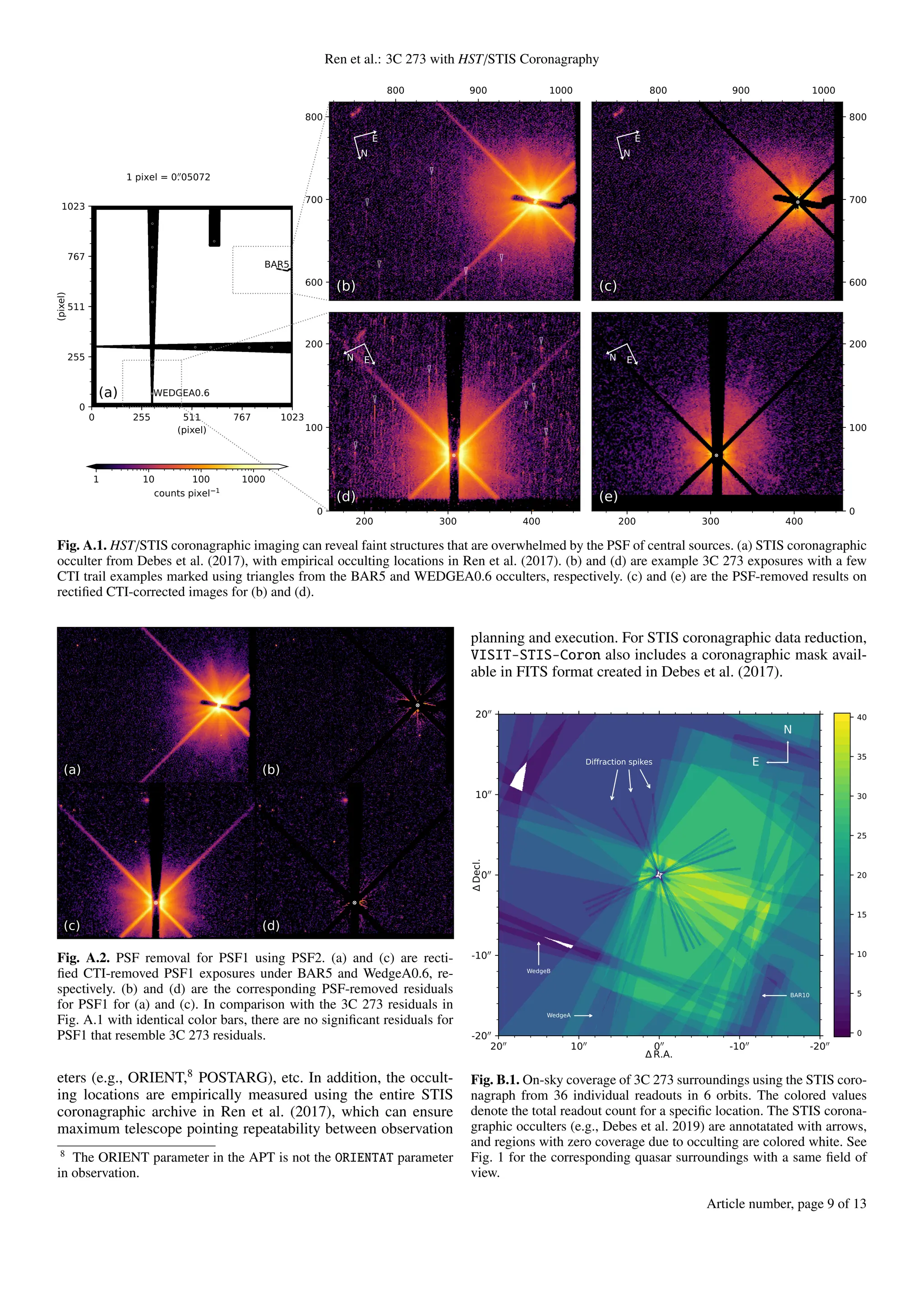
Using on-sky observations, we create the coverage map for
GO-16715 in Fig. B.1 that also takes into account of the diffrac-
tion spikes of the central quasar from HST optics. Despite a
nearly 360◦
azimuthal coverage, the north-east region of the
quasar surroundings has less exposures, which was not originally
planned in the Phase II, but instead due to an update3
in the HST
guide star catalog in 2022 between the two sets of 3C 273 visits.
-6000
-4000
-2000
000
2000
4000
6000
R.A.
-6000
-4000
-2000
000
2000
4000
6000
Decl.
2MASS J12290786+0203359
2MASS J12290318+0203185
10 1
100
101
102
[×10
20
erg
s
1
cm
2
Å
1
]
Fig. B.2. Full-frame result of 3C 273 surroundings from GO-16715. The
regions within the four dashed circles are used to estimate the noise.
-2000
-1000
000
1000
2000
R.A.
-2000
-1000
000
1000
2000
Decl.
+
E
N
0.1
1
10
100
1000
[S/N]
Fig. B.3. Pixel-wise S/N map, obtained through dividing Fig. 1 by the
pixel-wise standard deviation of the astrophysical-signal-free regions
identified by eye.
B.2. Signal-to-noise map
We calculate the pixel-wise signal-to-noise (S/N) map for Fig. 1
as follows. First we identify four background regions which do
not contain astrophysical signals by eye, see the full-frame re-
sult in Fig. B.2. We then calculate the standard deviation of the
selected regions to estimate the noise. The noise level does not
change significantly when we used only a few regions for analy-
sis or changed their locations and sizes. We finally divide Fig. 1
by that calculated value of standard deviation for these back-
ground regions, and present the S/N map in Fig. B.3.
To investigate the impact of the selection of background
regions, we have changed the locations and sizes selected re-
gions for noise estimation, and the resulting S/N maps do not
have significant change from Fig. B.3. In fact, due to the po-
sitions of the BAR5 and WedgeA0.6 occulters, the telescope
roll angles, and our readout in the full frame, the final full-
frame result has a field of view of ∼100′′
× 100′′
. In compari-
son, the 3C 273 host resides within a 40′′
× 40′′
region in Fig. 1
which is cropped from the full-frame result. As a result, while
there are foreground stars (2MASS J12290318+0203185 and
2MASS J12290786+0203359, which are located at 644 ± 7 pc
and 203.4 ± 1.9 pc from the Sun in Gaia DR3, respectively. The
two are not shown in Fig. 1 but available in the corresponding
full-frame image in Fig. B.2) and background galaxies in the
full-frame result, which can reach a large fraction of the areas in
a 120′′
×120′′
field, the majority of the full-frame result contains
background regions that can be used to quantify the noise in the
reduction.
B.3. Small scale features
We present in Fig. B.4 the small-scaled features identified in
Fig. 2 at different telescope orientations and occulting locations.
We present the surface brightness for the newly identified fea-
tures, as well as those in Martel et al. (2003), from Fig. 2 in
Table B.1.
Table B.1. Surface brightness of structures in Fig. 2
Feature Surface Brightness
(×10−20
erg s−1
cm−2
Å−1
)
b1 ∼0.5
b2 ∼0.3
b3 ∼0.3
CB 5 ± 2
CC 14 ± 5
CJ 3 ± 2
filament ∼0.4
E1 ∼0.6
JC 0.37 ± 0.17
IJ 0.25 ± 0.13
background 0.013 ± 0.013
Appendix C: Jet motion measurement
We assume that the surface brightness distribution of an elliptical
component follows a bivariate normal distribution,
S (r0) ∼ N2 (µ0, Σ0) , (C.1)
where Nk denotes a normal distribution with dimension k ∈ Z,
r0 = [x, y]T
∈ R2×1
denotes the on-sky location, µ0 ∈ R2×1
and
Σ0 ∈ R2×2
are the expectation and covariance matrix for the dis-
tribution, respectively. We can perform matrix translation then
rotation to obtain a new surface brightness distribution S ′
.
Article number, page 10 of 13

11. Ren et al.: 3C 273 with HST/STIS Coronagraphy
+ b1
b2
b3
+
+ +
200
0 -200
200
0
-200
+
200
0 -200
+
Fig. B.4. Small scale features in isophote-removed residuals in Fig. 2
can persist in multiple telescope orientations. (a), (c), and (e) are for
BAR5. (b), (d), and (f) are for WedgeA0.6.
C.1. Elliptical component motion
To enable the translation and rotation of the surface brightness
distribution in Eq. (C.1), we define r = [r⊤
0 , 1]⊤
to be a 3×1 col-
umn matrix, where ⊤
denotes matrix transpose. We additionally
define its corresponding expectation and covariance matrices to
be
µ = µ0 ⊕ 1, (C.2)
and
Σ = Σ0 ⊕ 0, (C.3)
respectively, where ⊕ is matrix direct sum. With these, we can
rewrite Eq. (C.1) in a 3-dimensional form,
S (r) ∼ N3 (µ, Σ) . (C.4)
For a translation matrix T, we have
T =








1 0 tx
0 1 ty
0 0 1







 ,
where tx ∈ R and ty ∈ R denote the translation along the x-
direction and y-direction, respectively. For a rotation matrix R,
we have
R =








cos tθ − sin tθ 0
sin tθ cos tθ 0
0 0 1







 ,
where tθ ∈ [−π, π) denotes the clockwise rotation about the ori-
gin. A translation then rotation a surface brightness distribution
following Eq. (C.4) then follows
S ′
(r) = RTS (r) ∼ N3
RTµ, RTΣT⊤
R⊤
.
Given that the last row and column of Eq. (C.3) are composed of
0, we can rewrite the above distribution as
S ′
(r) ∼ N3
RTµ, RΣR⊤
. (C.5)
C.2. Motion quantification
0.0
0.2
0.4
0.6
0.8
1.0
0.0
0.2
0.4
0.6
0.8
1.0
0.00
5 0 -0.00
5
0.00
5
0
-0.00
5
0.00
5 0 -0.00
5
0.4
0.2
0.0
0.2
0.4
Fig. C.1. Ellipse fitting to obtain the morphology and motion for jet
component A2. The (a) 2000 and (b) 2022 data are normalized to have
a peak count of one in each panel. (c) and (d) are the best-fit models,
which follow identical bivariate normal distribution but with location
offset, for (a) and (b), respectively. (e) and (f) are the residuals after
subtracting the models from the corresponding data.
For a bivariate normal distribution at two epochs, we assume
that its morphology does not change significantly. In this way, we
can use Eqs. (C.4) and (C.5), which share identical morpholog-
ical parameters µ and Σ, to obtain the relative motion between
Article number, page 11 of 13

12. AA proofs: manuscript no. ms
two epochs. To maximize the information from both datasets,
we use the statistical concept of dummy variables (see, e.g., Ren
et al. 2020, for an application in high-contrast imaging science)
to fit Eqs. (C.4) and (C.5) simultaneously.
First, we rewrite the distribution of the first two entries in
Eqs. (C.4) in a general form in Cartesian coordinates, with the
distribution centered at (x0, y0) and rotated θ0 ∈ [−π, π) along the
counterclockwise rotation from a rectangular bivariate normal
distribution. We have
S (x, y) = A exp
(
−
1
2
h
a(x − x0)2
+ 2b(x − x0)(y − y0) + c(y − y0)2
i)
,
(C.6)
where A ∈ R is the amplitude, and















a = cos2
θ0
σ2
x
+ sin2
θ0
σ2
y
b = −sin 2θ0
2σ2
x
+ sin 2θ0
2σ2
y
c = sin2
θ0
σ2
x
+ cos2
θ0
σ2
y
. (C.7)
Second, we introduce a dummy variable D ∈ {0, 1} to
Eq. (C.6) to denote the offset along x- and y-axis, and rotation
from θ0 using the following substitution









x0 ≡ x0 + txD
y0 ≡ y0 + tyD
θ0 ≡ θ0 + tθD
, (C.8)
to obtain the general form for the first two entries in Eq. (C.5)
when D = 1.
Third, combining Eqs. (C.6)–(C.8), we can obtain the gen-
eral form for the first two entries in Eq. (C.4) when the dummy
variable D = 0, and the two in Eq. (C.5) when D = 1. To ob-
tain the morphological and offset parameters in two epochs, we
now use (x, y, D) as the input independent variables, and surface
brightness S (x, y, D) as the dependent variable.
For each elliptical component, using the curve_fit func-
tion from scipy (Virtanen et al. 2020), we can obtain the best-fit
parameters for the elliptical morphology (i.e., A, x0, y0, σx, σy,
θ0) and the motion (i.e., tx, ty, tθ), as well as their covariance ma-
trix. In practice, we also had a local background brightness value
that is added to Eq. (C.6) to quantify the background difference
in two epochs. We adopt the square root of the diagonal values
of the covariance matrix from curve_fit as the uncertainty of
the elliptical and motion parameters. We present in Fig. C.1 a
demonstration of the fitting process.
C.3. Instrument offset calibration
To address potential bias in our alignment and rotation of two
images in 2000 and 2022, we use background objects to cal-
ibrate the translation and rotation offsets between two epochs,
see Fig. C.2. Assuming the background sources in the two im-
ages do not move, then we can first offset then rotate one image
to another to calibrate the global offset.
For a background object, we can follow Appendix C.2 to ob-
tain its best-fit and uncertainty values for the motion parameters:
tx, ty, and tθ. To quantify the global offset in ˆ
tx, ˆ
ty, and ˆ
tθ, we
assume that the motion parameters are dependent on the centers
of the ellipses (x0, y0). Using the odr function which performs
10 3
10 2
10 1
100
[counts
s
1
pixel
1
]
Fig. C.2. Components (marked by squares) and background objects
(marked with diamonds) used in motion measurement and instrument
offset calibration, respectively.
orthogonal least-squared-fitting for data with both input and out-
put uncertainties (Boggs et al. 1989) from scipy, we obtained
the best-fit parameters for ˆ
tx, ˆ
ty, and ˆ
tθ.
For a jet component, we followed Appendix C.2 to obtain
its offset, then corrected the global offset measured from back-
ground objects. To obtain the jet component motion along the jet
direction, we first obtained the position angle of the jet by per-
forming least-square fit to the location of the jet components. We
then projected the calibrated offset for a jet component, which is
expressed as a bivariate normal distribution from the odr out-
puts, to the jet direction though matrix rotation, see Eq. (B8) in
Shuai et al. (2022) for a similar approach.
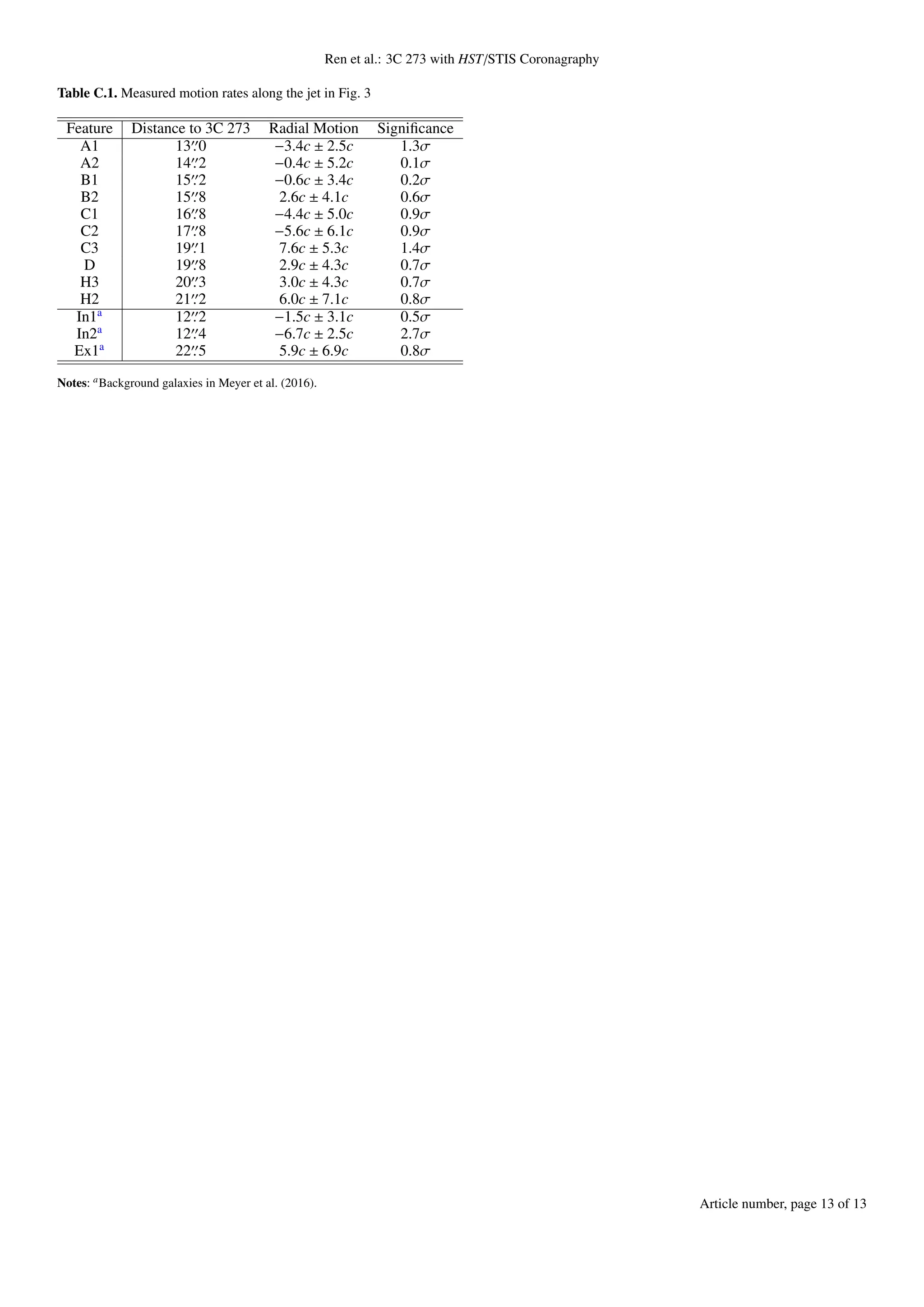
C.4. Measured motion
We present the measured motion rates from Sect. 3.2 in Ta-
ble C.1.
Article number, page 12 of 13

13. Ren et al.: 3C 273 with HST/STIS Coronagraphy
Table C.1. Measured motion rates along the jet in Fig. 3
Feature Distance to 3C 273 Radial Motion Significance
A1 13′′
.0 −3.4c ± 2.5c 1.3σ
A2 14′′
.2 −0.4c ± 5.2c 0.1σ
B1 15′′
.2 −0.6c ± 3.4c 0.2σ
B2 15′′
.8 2.6c ± 4.1c 0.6σ
C1 16′′
.8 −4.4c ± 5.0c 0.9σ
C2 17′′
.8 −5.6c ± 6.1c 0.9σ
C3 19′′
.1 7.6c ± 5.3c 1.4σ
D 19′′
.8 2.9c ± 4.3c 0.7σ
H3 20′′
.3 3.0c ± 4.3c 0.7σ
H2 21′′
.2 6.0c ± 7.1c 0.8σ
In1a
12′′
.2 −1.5c ± 3.1c 0.5σ
In2a
12′′
.4 −6.7c ± 2.5c 2.7σ
Ex1a
22′′
.5 5.9c ± 6.9c 0.8σ
Notes: aBackground galaxies in Meyer et al. (2016).
Article number, page 13 of 13