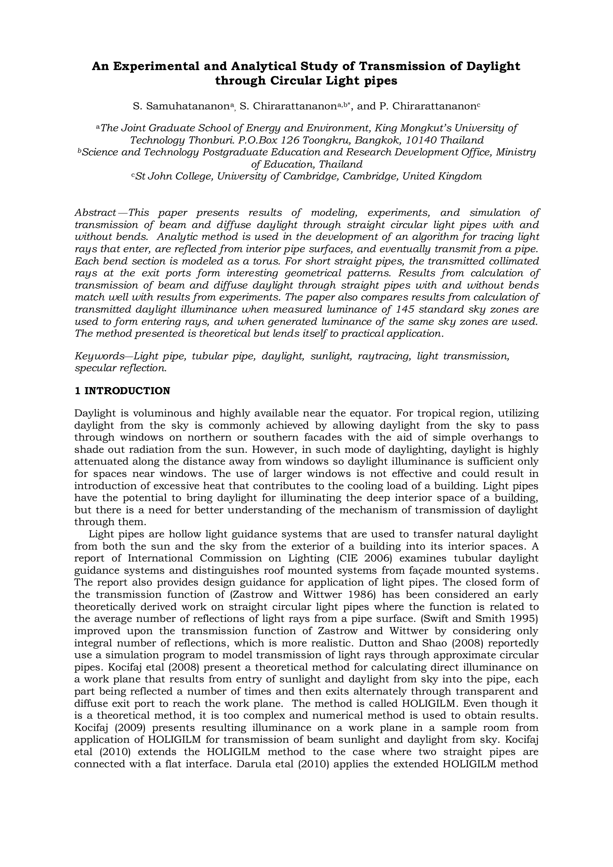
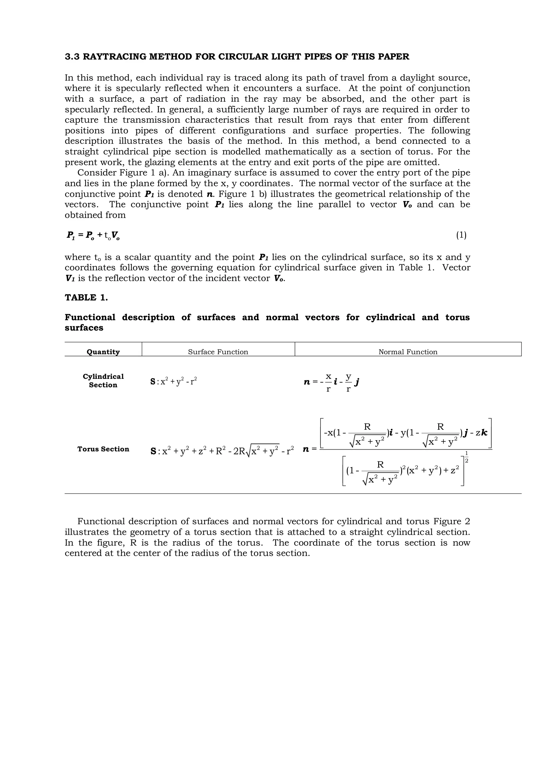
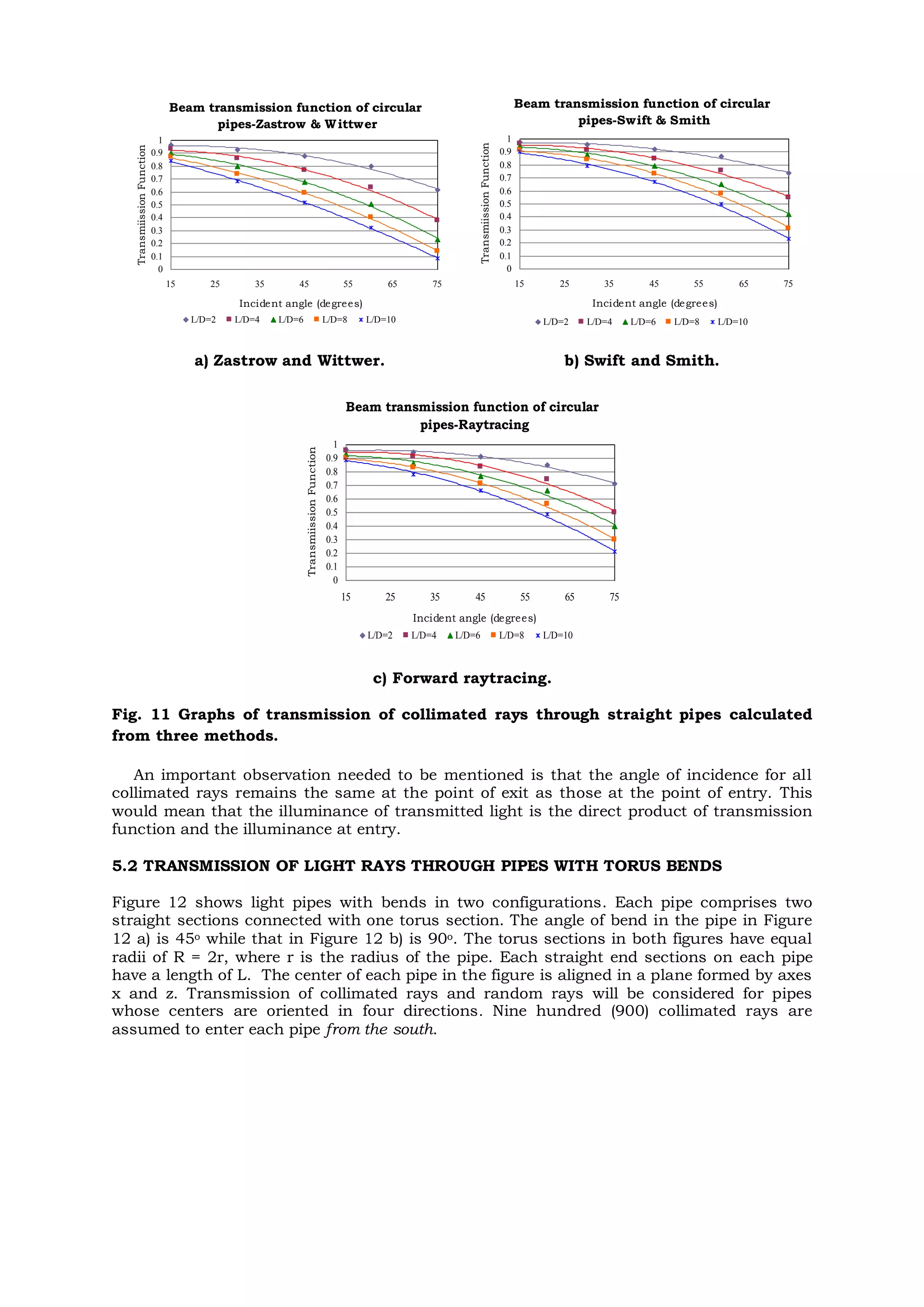
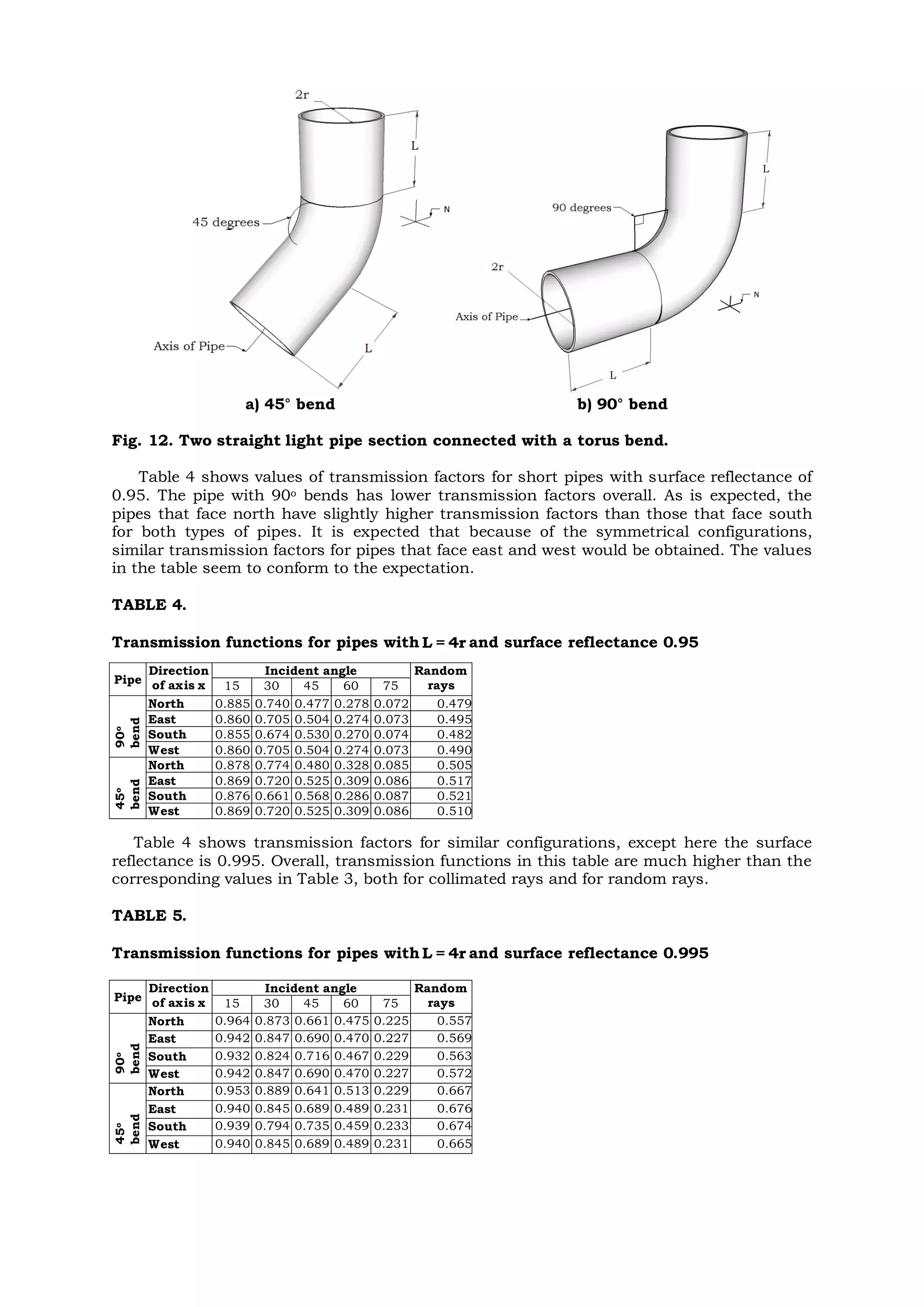
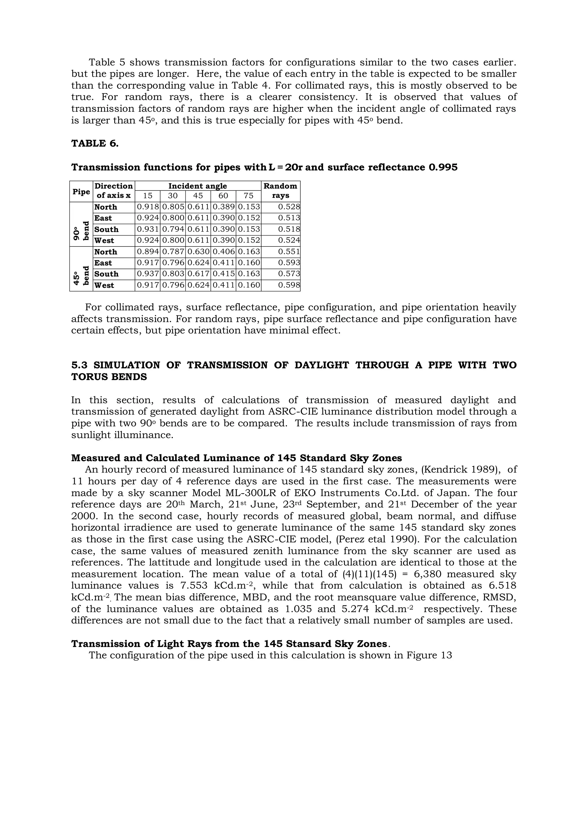
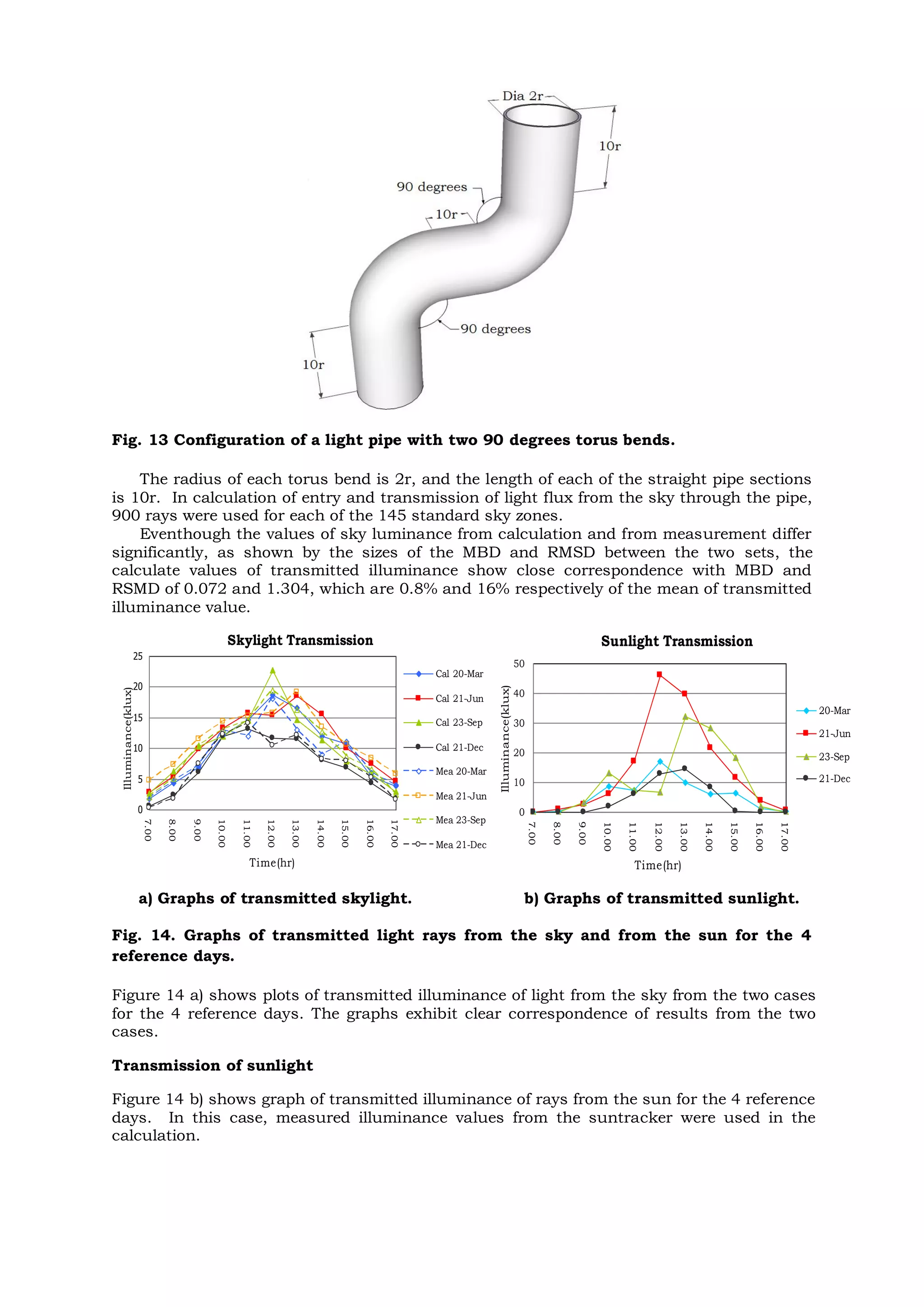
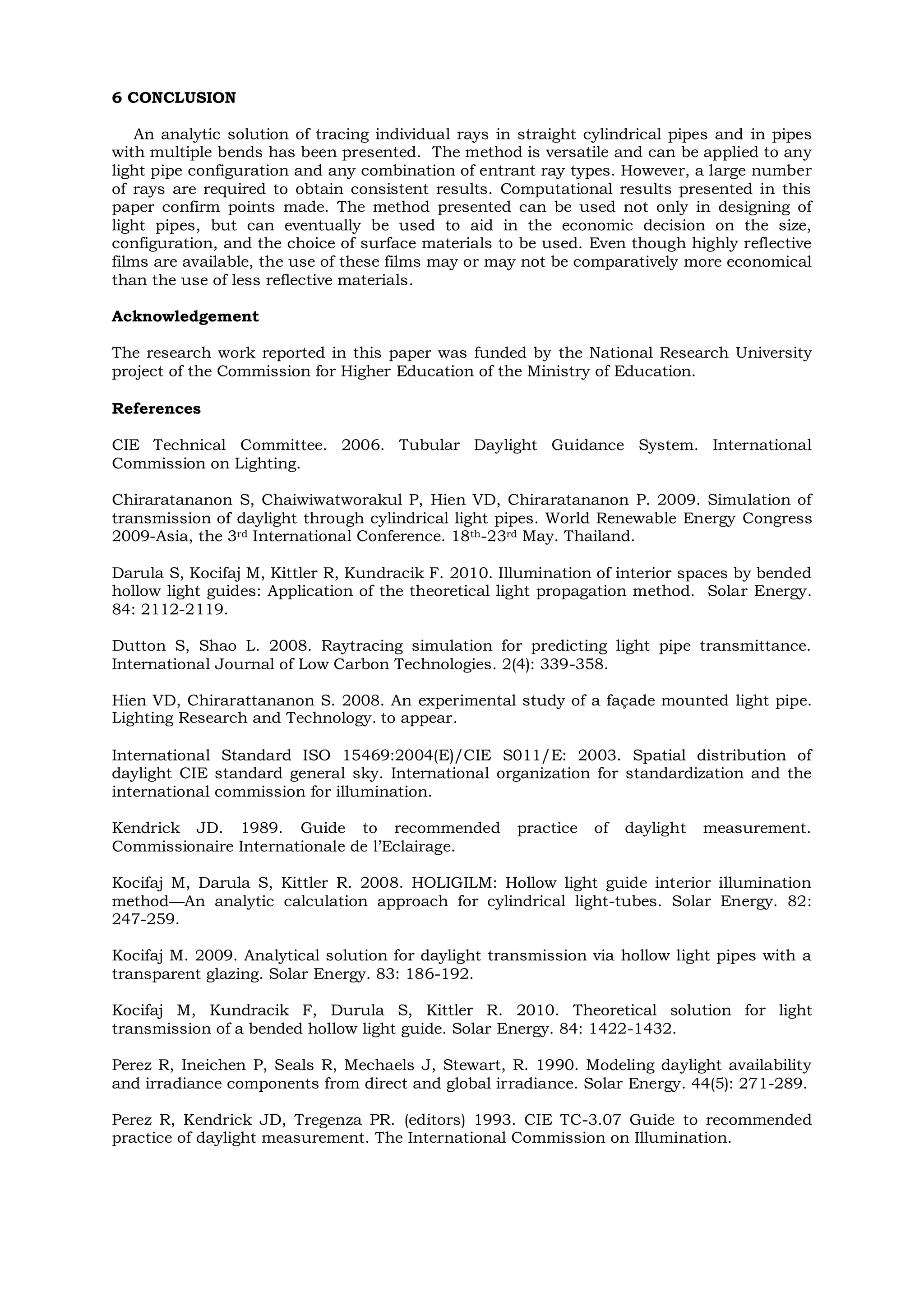
This document presents the results of a study on modeling and simulating the transmission of daylight through circular light pipes with and without bends. It describes an analytical raytracing method developed to compute the transmission of collimated and diffuse light through such pipes. Experimental results on light transmission through straight pipes and pipes with bends are shown to match well with calculations. The paper also compares transmitted daylight illuminance values using measured versus generated sky luminance data as light inputs.

2. An Experimental and Analytical Study of Transmission of Daylight
through Circular Light pipes
S. Samuhatananona
, S. Chirarattananona,b*, and P. Chirarattananonc
aThe Joint Graduate School of Energy and Environment, King Mongkut’s University of
Technology Thonburi. P.O.Box 126 Toongkru, Bangkok, 10140 Thailand
bScience and Technology Postgraduate Education and Research Development Office, Ministry
of Education, Thailand
cSt John College, University of Cambridge, Cambridge, United Kingdom
Abstract —This paper presents results of modeling, experiments, and simulation of
transmission of beam and diffuse daylight through straight circular light pipes with and
without bends. Analytic method is used in the development of an algorithm for tracing light
rays that enter, are reflected from interior pipe surfaces, and eventually transmit from a pipe.
Each bend section is modeled as a torus. For short straight pipes, the transmitted collimated
rays at the exit ports form interesting geometrical patterns. Results from calculation of
transmission of beam and diffuse daylight through straight pipes with and without bends
match well with results from experiments. The paper also compares results from calculation of
transmitted daylight illuminance when measured luminance of 145 standard sky zones are
used to form entering rays, and when generated luminance of the same sky zones are used.
The method presented is theoretical but lends itself to practical application.
Keywords—Light pipe, tubular pipe, daylight, sunlight, raytracing, light transmission,
specular reflection.
1 INTRODUCTION
Daylight is voluminous and highly available near the equator. For tropical region, utilizing
daylight from the sky is commonly achieved by allowing daylight from the sky to pass
through windows on northern or southern facades with the aid of simple overhangs to
shade out radiation from the sun. However, in such mode of daylighting, daylight is highly
attenuated along the distance away from windows so daylight illuminance is sufficient only
for spaces near windows. The use of larger windows is not effective and could result in
introduction of excessive heat that contributes to the cooling load of a building. Light pipes
have the potential to bring daylight for illuminating the deep interior space of a building,
but there is a need for better understanding of the mechanism of transmission of daylight
through them.
Light pipes are hollow light guidance systems that are used to transfer natural daylight
from both the sun and the sky from the exterior of a building into its interior spaces. A
report of International Commission on Lighting (CIE 2006) examines tubular daylight
guidance systems and distinguishes roof mounted systems from façade mounted systems.
The report also provides design guidance for application of light pipes. The closed form of
the transmission function of (Zastrow and Wittwer 1986) has been considered an early
theoretically derived work on straight circular light pipes where the function is related to
the average number of reflections of light rays from a pipe surface. (Swift and Smith 1995)
improved upon the transmission function of Zastrow and Wittwer by considering only
integral number of reflections, which is more realistic. Dutton and Shao (2008) reportedly
use a simulation program to model transmission of light rays through approximate circular
pipes. Kocifaj etal (2008) present a theoretical method for calculating direct illuminance on
a work plane that results from entry of sunlight and daylight from sky into the pipe, each
part being reflected a number of times and then exits alternately through transparent and
diffuse exit port to reach the work plane. The method is called HOLIGILM. Even though it
is a theoretical method, it is too complex and numerical method is used to obtain results.
Kocifaj (2009) presents resulting illuminance on a work plane in a sample room from
application of HOLIGILM for transmission of beam sunlight and daylight from sky. Kocifaj
etal (2010) extends the HOLIGILM method to the case where two straight pipes are
connected with a flat interface. Darula etal (2010) applies the extended HOLIGILM method

3. to obtain illuminance values and patterns at the exit port and at the work plane in a sample
room.
This paper presents an analytical method that utilizes forward raytracing principle to the
development of a procedure for computation of transmission of collimated light rays and
randomly emitted (diffuse) light through circular mirror light pipes (CMLP) with and without
bends. Section 2 of this paper reviews theoretically derived light transmission models from
literatures. Section 3 presents the development of the procedure for computation of
transmission of light rays through light pipes. Section 4 presents comparative results from
calculation and from outdoor physical experiment on transmission of collimated sun rays
and daylight from the sky through light pipes. Section 5 presents further results from
calculation and from simulating transmission of sunlight and daylight from the sky. Section
6 concludes the paper.
2 THEORETICALLY DERIVED TRANSMISSION FUNCTIONS FOR STRAIGHT PIPE
Consider a light ray entering a straight circular light pipe in Figure 1.
a) A perspective view b) A plan view
Fig. 1. The geometry of a ray entering a model of circular light pipe.
A light ray enters the entry port of the pipe at position Po. The ray travels in the direction
represented by the unit vector Vo. The ray reaches point P1 on the pipe surface and the
reflected ray represented by vector V1 reaches the pipe surface at another point P2. The
length of the projection of vector V1 onto the x-y plane is d.
2.1 TRANSMISSION FUNCTION OF ZASTROW AND WITTWER
Zastrow and Wittwer (1986) define the average length of projection of the reflection vectors
on the x-y plane as deff. If the length of the pipe is L and the incident angle of the light ray
with respect to the pipe isθ , then the approximate number of reflections of the ray from the
surface is
eff eff
L Ltanθ
=
d d
tanθ
The authors derive deff from a consideration of the average length of the projected vector
as
eff
πD πr
d = =
4 2
where D is the diameter of the light pipe and r is the radius of the pipe. If the reflectance of
the surface of the pipe is , then the transmission function T, the ratio of the radiative
power of the transmitted ray to that of the entering ray, is obtained as
eff
Ltanθ
d
T = ρ

4. This relationship was shown by (Swift and Smith 1995) to be only valid for pipes with
high aspect ratios (larger value of the ratio of pipe length to pipe diameter), small incident
angles, and high surface reflectance.
2.2 TRANSMISSION FUNCTION OF SWIFT AND SMITH
Swift and Smith (1995) consider the transmission function of (Zastrow and Wittwer 1986) to
be an approximation and develop an exact analytical expression to be used instead. The
expression is:

1 ptanθ2
int[ ]
s
2
s=0
4 s ptanθ
T = ρ (1-(1- ρ)(-int[ ]))ds
π s1- s
where
L
p =
D
, is the aspect ratio or the length to diameter ratio, and where int[x] denotes
the integer part of x. This function T represents the average transmission for light rays that
are collimated in one direction.
3 RAYTRACING FOR STRIGHT PIPES AND PIPES WITH BENDS
The raytracing method is based on tracing of specular reflection of individual rays.
3.1 APPLICATION OF RAYTRACING TO RECTANGULAR PIPES
Raytracing has been applied successfully to the study of façade-mounted rectangular pipes
by (Hien and Chirarattananon 2008). (Dutton and Shao 2008), use long thin rectangular
sections to form approximate circular shaped pipes and simulate light pipe transmission by
the use of Photopia, a computer program. When the authors simulate the transmission of
collimated rays, the results from Photopia calculation match very well with those calculated
from the transmission function of (Swift and Smith 1995).
3.2 BACKWARD RAYTRACING METHOD FOR CIRCULAR LIGHT PIPES
Kocifaj etal (2008) develop a method called HOLIGILM for calculation of illuminance on an
incremental area at the exit port of a circular light pipe by considering backward tracing of
a light ray through the entry dome or port to a sky zone. For the same incremental area,
rays from all directions are traced until light fluxes from all zones of the sky and light flux
from the sun (if present) are accounted. Light fluxes from the sky zones and sun contribute
to the illuminance of the incremental area. Light flux passing the incremental area at the
exit port constitutes exitance from the area and is then used to calculate luminance,
intensity, and eventually the illuminance on an area on the work plane in a given room.
Kocifaj (2009) illustrates numerical results from the method and notes that for relatively
long pipes, ‘distorted image of the sun is spread over a circular region in the work plane’.
The author also reports the use of the method for calculation of transmission of beam
sunlight and daylight under clear and cloudy sky using two standard CIE sky luminance
distributions, (CIE 2003). Both transparent and diffuse optical components are used
alternately at the exit port.
Kocifaj etal (2010) extends the HOLIGILM method to the case where two straight circular
pipes are connected at an angle at a flat interface, where the shape of the interface becomes
elliptical. Darula etal (2010) illustrates results from the use of the extended method. Here,
the authors also note the existence of a circular region on the work plane due to
transmission of light from the sun. The authors also note that their method is fast, but the
speed and precision of calculation depends on the fineness of a ‘grid’ used.
The reports of (Darula etal 2010) and of (Kocifaj 2009) show that there is a circular band
on the work plane in the sample room from transmission of beam sunlight through a pipe,
be it a single straight pipe or two straight pipes connected to form a single pipe.

5. 3.3 RAYTRACING METHOD FOR CIRCULAR LIGHT PIPES OF THIS PAPER
In this method, each individual ray is traced along its path of travel from a daylight source,
where it is specularly reflected when it encounters a surface. At the point of conjunction
with a surface, a part of radiation in the ray may be absorbed, and the other part is
specularly reflected. In general, a sufficiently large number of rays are required in order to
capture the transmission characteristics that result from rays that enter from different
positions into pipes of different configurations and surface properties. The following
description illustrates the basis of the method. In this method, a bend connected to a
straight cylindrical pipe section is modelled mathematically as a section of torus. For the
present work, the glazing elements at the entry and exit ports of the pipe are omitted.
Consider Figure 1 a). An imaginary surface is assumed to cover the entry port of the pipe
and lies in the plane formed by the x, y coordinates. The normal vector of the surface at the
conjunctive point P1 is denoted n. Figure 1 b) illustrates the geometrical relationship of the
vectors. The conjunctive point P1 lies along the line parallel to vector Vo and can be
obtained from
ot1 o oP = P + V (1)
where to is a scalar quantity and the point P1 lies on the cylindrical surface, so its x and y
coordinates follows the governing equation for cylindrical surface given in Table 1. Vector
V1 is the reflection vector of the incident vector Vo.
TABLE 1.
Functional description of surfaces and normal vectors for cylindrical and torus
surfaces
Quantity Surface Function Normal Function
Cylindrical
Section
Torus Section
Functional description of surfaces and normal vectors for cylindrical and torus Figure 2
illustrates the geometry of a torus section that is attached to a straight cylindrical section.
In the figure, R is the radius of the torus. The coordinate of the torus section is now
centered at the center of the radius of the torus section.
2 2 2
: x + y - rS
x y
= - -
r r
n i j
2 2 2 2 2 2 2
: x + y + z + R - 2R x + y - rS
2 2 2 2
1
2
2 2 2 2
2 2
R R
-x(1- ) - y(1- ) - z
x + y x + y
=
R
(1- ) (x + y )+ z
x + y
 
 
  
 
 
  
i j k
n

6. Fig. 2. Geometry of a torus section that is attached between two straight circular
sections.
In the figure, the point of entry to the torus section Pc, the entry vector Vt, the
conjunctive point Pt, the normal vector nt, and the reflection vector Vr corresponds to those
of the straight cylindrical section in Figure 1. In Figure 1 and Figure 2 the components of
the reflection vectors and the scalar quantity to constitute four unknown variables in each
case. The surface function and application of the rule of specular reflection gives four
equations that can be used to solve for the values of the four variables in each case.
Conceptually, the method in this paper is similar to the backward raytracing method of
(Kocifaj etal 2008) and its extension. However, daylight from the sky and sun in this paper
is decoupled from the pipe. As seen in Section 4 and 5, measured data of sky luminance in
standard sky zones could be used as input instead of values calculated from luminance
models. For the present work, a bend is also modelled as a torus section which is
distinctively different from that of (Kocifaj etal 2008).
Uniform Entry and Emission of Rays
One common option in the calculation of entry of light rays into the entry aperture of a
circular pipe is to assume that the rays enter uniformly over the aperture. This means that
each ray enters into an equally divided small area on the aperture. The following procedure
illustrates a method of dividing a circular area into equal small areas. Consider the circular
area and the small concentric rings in Figure 3 a).
a) Division of concentric ring. b) The centers of 900 equal subareas.
Fig. 3. Division of a circular area into 900 equal subareas.
r1
r2




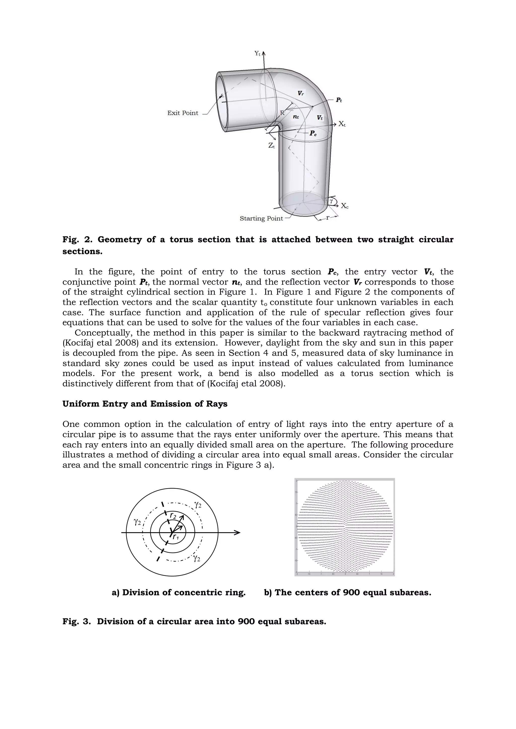
7. The innermost ring has a radius of r1. The area of this circle is
2
2πr
1
. The next circle has a
radius 2 1r = 2r . The subsequent circles have radii of 3 1 n 1r = 3r ,…,r = nr . This means that the
successive rings have the following areas,
2 2 2
2 1 1
2 2 2 2
n 1 1
r : 2πr [2 -1] = 3(2πr ),
r : 2πr [(n) - (n -1) ] = (2n -1)(2πr ).
To obtain equal small incremental areas, the area of the ring between the circles of
radius r1 and r2 is divided into 3 equal areas. The angle 2γ in Figure 3 then equals
2π
3
. For
the ring between the circles of radii ri-1 and ri, the size of the corresponding angle iγ
equals
2π
2i -1
. The number of the small equal areas sums to n2. Figure 3 b) illustrates the
points of entry of each ray into the entry port of a pipe.
Random Rays
The elevation angle and the azimuth angle of a unit vector that represents a ray
randomly emitted from a diffuse surface are obtained from, (Tregenza 1993),
, and
,
sinθ = R
1
= 2πR
2

where R1 and R2 are random numbers each with a value between 0 and 1.
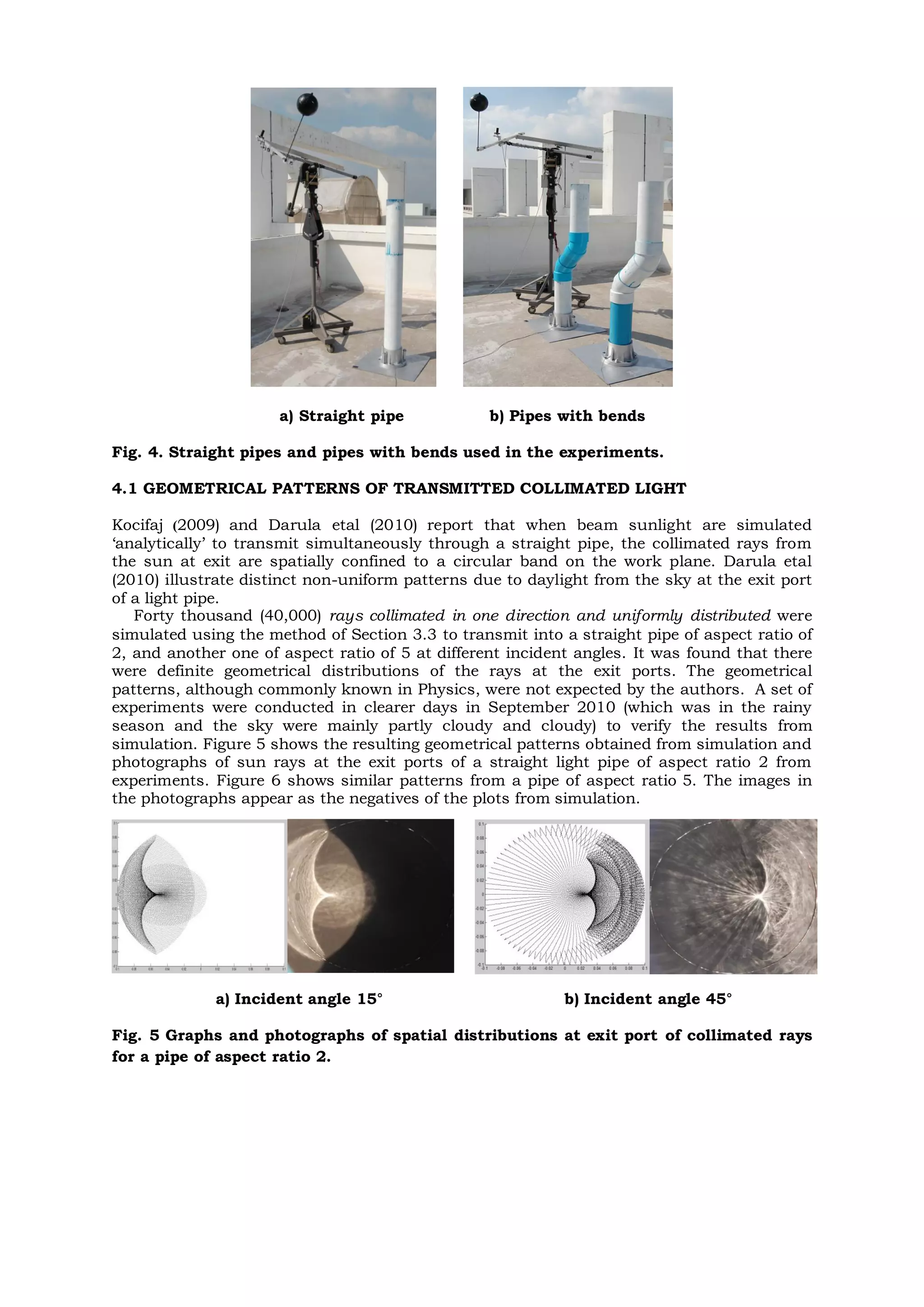
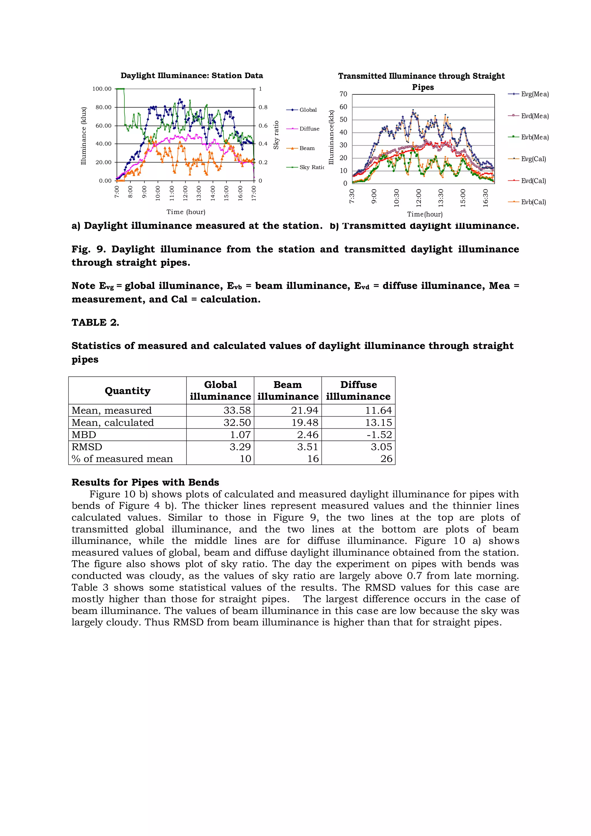
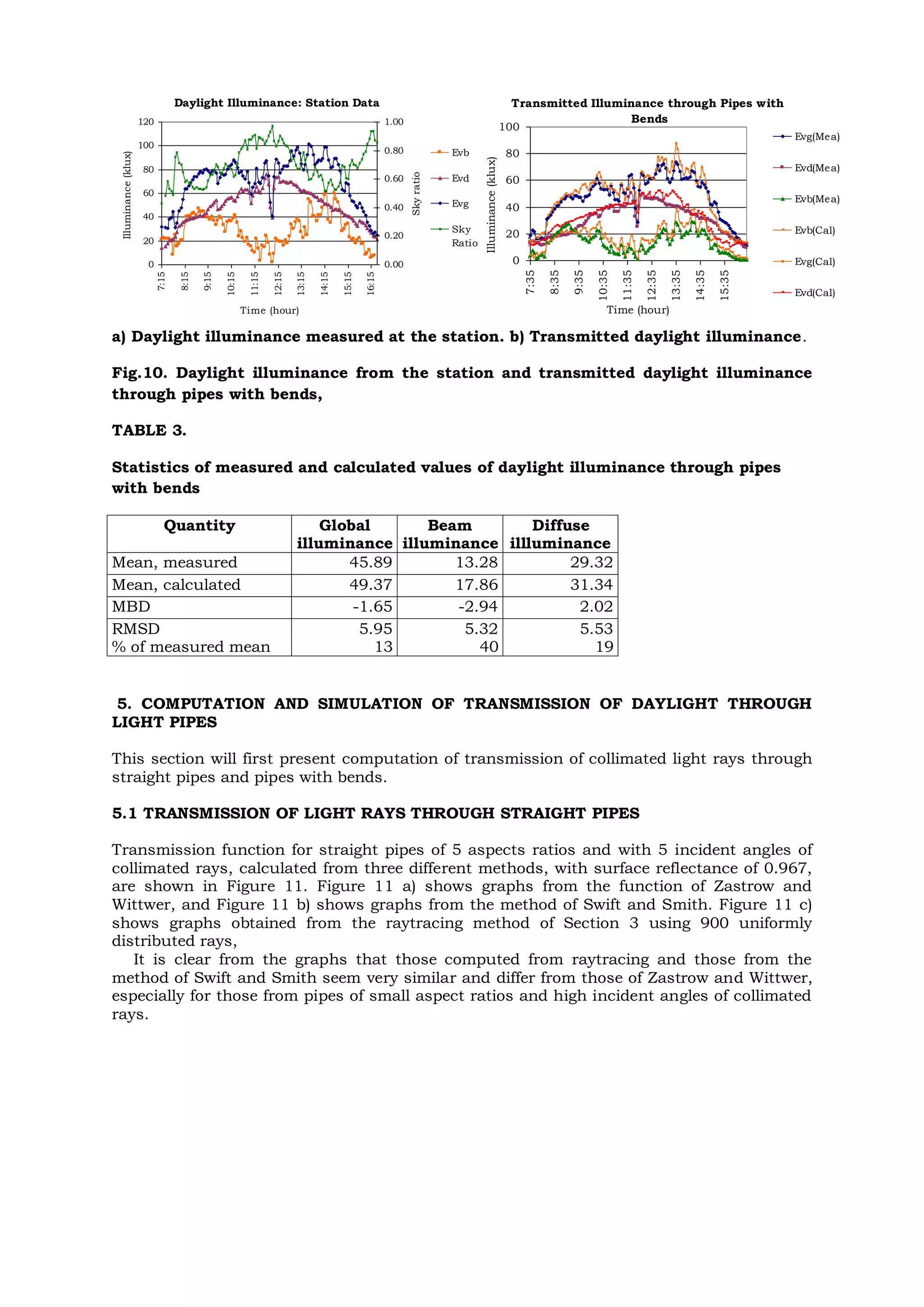
4 COMPUTATIONAL AND EXPERIMENTAL RESULTS
We first examine results from computation and from physical experiment of light
transmission through straight pipes and pipes with bends. In the computation to be
described, the rays are emitted uniformly into the entry aperture of circular light pipes in
accordance with the method of Section 3.3. This is in contrast to that in (Chiraratananon
etal 2009) that uses randomly distributed rays. The authors are convinced that for limited
number of rays, the method used here produces more consistent results.
A set of light pipes were fabricated from polyvinyl chloride (pvc) pipes commonly used in
domestic plumbing. The diameters of the pipes are 150 mm. Bend sections from pvc pipes
are used as torus bends for the light pipes. The inner surfaces of all pipe sections were
lined manually with Daylighting Film of 3M Inc., USA. The film has a reflectance greater
than 0.99 as given in the specification. The surfaces of the finished pipes, especially the
bend sections, are not expected to be as reflective as that of the original film. Figure 4
shows photographs of the straight pipes and pipes with two 450 bends.

8. a) Straight pipe b) Pipes with bends
Fig. 4. Straight pipes and pipes with bends used in the experiments.
4.1 GEOMETRICAL PATTERNS OF TRANSMITTED COLLIMATED LIGHT
Kocifaj (2009) and Darula etal (2010) report that when beam sunlight are simulated
‘analytically’ to transmit simultaneously through a straight pipe, the collimated rays from
the sun at exit are spatially confined to a circular band on the work plane. Darula etal
(2010) illustrate distinct non-uniform patterns due to daylight from the sky at the exit port
of a light pipe.
Forty thousand (40,000) rays collimated in one direction and uniformly distributed were
simulated using the method of Section 3.3 to transmit into a straight pipe of aspect ratio of
2, and another one of aspect ratio of 5 at different incident angles. It was found that there
were definite geometrical distributions of the rays at the exit ports. The geometrical
patterns, although commonly known in Physics, were not expected by the authors. A set of
experiments were conducted in clearer days in September 2010 (which was in the rainy
season and the sky were mainly partly cloudy and cloudy) to verify the results from
simulation. Figure 5 shows the resulting geometrical patterns obtained from simulation and
photographs of sun rays at the exit ports of a straight light pipe of aspect ratio 2 from
experiments. Figure 6 shows similar patterns from a pipe of aspect ratio 5. The images in
the photographs appear as the negatives of the plots from simulation.
a) Incident angle 15° b) Incident angle 45°
Fig. 5 Graphs and photographs of spatial distributions at exit port of collimated rays
for a pipe of aspect ratio 2.

9. a) Incident angle 15° b) Incident angle 45°
Fig. 6 Graphs and photographs of spatial distributions at exit port from collimated
rays for a pipe of aspect ratio 5.
At higher incident angles and for pipes with higher aspect ratios, the distributions
become more uniform as is evident in Figure 6 b). For rays that are emitted in random
directions, the pattern at the exit port also shows random distribution, as shown in Figure
7. The results from the cases reported here does not seem to correspond to what was
observed by Kocifaj (2009).
Fig. 7. Spatial distribution at exit aperture from random rays through straight pipe of
aspect ratio 5.
4.2 EXPERIMENTAL AND COMPUTATIONAL RESULTS OF DAYLIGHT TRANSMISSION
A series of experiments were conducted in the latter part of 2010 and early 2011 to obtain
transmission functions of direct sunlight and diffuse daylight from the sky for light pipes of
specular surfaces. Some selected experimental results are reported here with
computational results.
Arrangement of Experiments
In order to obtain separate experimental transmission functions for sunlight and for light
from the sky, two identical straight pipes of aspect ratio 10 were used. A shading ball was
attached to a sun tracking device. The ball was used to shade sunlight from the entry port
of one pipe. The sun tracker and the shading ball are visible in Figure 4 a). The second
pipe was exposed to global illuminance from the sun and sky. The difference between the
measured values of transmitted global illuminance and transmitted diffuse illuminance
from the sky is the transmitted beam illuminance. Figure 4 b) shows an identical
arrangement for a pair of light pipes with bends.
Computation
Measured sunlight illuminance was used in the calculation of beam transmission using
the method described in Section 3. For calculation of transmission of diffuse daylight, the
ASRC-CIE sky luminance model was used, (Perez etal 1990). This model uses four CIE sky
models, clear, intermediate, overcast, and a high turbidity clear sky model. Perez’s
clearness index and brightness index are used to identify sky condition and to weight
contribution from each of the four CIE sky models. In utilizing this model, the values of
measured beam irradiance and diffuse irradiance are used to calculate the value of
clearness index and brightness index of Perez. Next, the values of relative luminance of 145
standard sky zones, each geometrically subtended a given solid angle, (Perez etal 1993), in
the sky hemisphere are calculated from the ASRC-CIE model. The model references zenith

10. luminance. The method described in Section 3 is then used to calculate transmission of
900 rays from each of the 145 standard sky zones of the sky hemisphere. The resulting
transmitted illuminance at the exit port from each point is summed to give total transmitted
illuminance of light from the sky. The values of beam sunlight illuminance and irradiance,
diffuse and global illuminance and irradiance, and zenith luminance are measured from
equipment in a station located near the experimental site.
The Daylight Measurement Station
A daylight measurement station has been set up on top of a 7-storey building in a
seaside campus of the university. Beam normal illuminance and irradiance are measured
directly by a suntracker. The tracker also holds two shading balls to shade out sunlight
and sun irradiance from an illuminance sensor and an irradiance sensor to give values of
diffuse sky illuminance and diffuse irradiance. Global illuminance and global irradiance as
well as total illuminance and total irradiance in each cardinal direction are measured by
individual sensors. There is also a zenith luminance sensor. All data are first logged in one-
minute interval and averaged and archived as 5-minute data. Figure 8 shows some
equipment from the station.
a) The sun tracker.
Fig. 8. Daylight and solar radiation measurement equipment at the station.
Results for Straight Pipes
Figure 9 b) shows plots of calculated and measured daylight illuminance for straight
pipes. The thicker lines represent measured values and the thinnier lines calculated values.
The two lines at the top are plots of transmitted global illuminance, and the two lines at the
bottom are plots of beam illuminance, while the middle lines are for diffuse illuminance.
Figure 9 a) shows the measured values of global, beam and diffuse daylight illuminance
obtained from the station. The figure also shows plot of sky ratio, the ratio of diffuse to
global illuminance. Since measured transmitted beam illuminance values are obtained as
the difference between the transmitted total illuminance and transmitted diffuse
illuminance values, the error of measured transmitted beam measurements can be as high
as the sum of errors from the other two. Table 2 shows some statistical values of the
results. The calculated mean transmitted beam illuminance values are higher than the
measured mean values while the opposite result is true for the diffuse illuminance. The
RMSD (root meansquare difference) values vary from 10% to 26% of the corresponding
mean values. The largest difference occurs in the case of diffuse illuminance. The sky was
mostly partly cloudy to cloudy throughout the duration of the experiment, as is evident
from an examination of the graph of the sky ratio and the pattern of the beam illuminance.
b) Sensors for measurement of total
illuminance and total irradiance.

11. a) Daylight illuminance measured at the station. b) Transmitted daylight illuminance.
Fig. 9. Daylight illuminance from the station and transmitted daylight illuminance
through straight pipes.
Note Evg = global illuminance, Evb = beam illuminance, Evd = diffuse illuminance, Mea =
measurement, and Cal = calculation.
TABLE 2.
Statistics of measured and calculated values of daylight illuminance through straight
pipes
Quantity
Global
illuminance
Beam
illuminance
Diffuse
illluminance
Mean, measured 33.58 21.94 11.64
Mean, calculated 32.50 19.48 13.15
MBD 1.07 2.46 -1.52
RMSD
% of measured mean
3.29
10
3.51
16
3.05
26
Results for Pipes with Bends
Figure 10 b) shows plots of calculated and measured daylight illuminance for pipes with
bends of Figure 4 b). The thicker lines represent measured values and the thinnier lines
calculated values. Similar to those in Figure 9, the two lines at the top are plots of
transmitted global illuminance, and the two lines at the bottom are plots of beam
illuminance, while the middle lines are for diffuse illuminance. Figure 10 a) shows
measured values of global, beam and diffuse daylight illuminance obtained from the station.
The figure also shows plot of sky ratio. The day the experiment on pipes with bends was
conducted was cloudy, as the values of sky ratio are largely above 0.7 from late morning.
Table 3 shows some statistical values of the results. The RMSD values for this case are
mostly higher than those for straight pipes. The largest difference occurs in the case of
beam illuminance. The values of beam illuminance in this case are low because the sky was
largely cloudy. Thus RMSD from beam illuminance is higher than that for straight pipes.
Daylight Illuminance: Station Data
0.00
20.00
40.00
60.00
80.00
100.00
7:00
8:00
9:00
10:00
11:00
12:00
13:00
14:00
15:00
16:00
17:00
Time (hour)
Illuminance(klux)
0
0.2
0.4
0.6
0.8
1
Skyratio
Global
Diffuse
Beam
Sky Ratio
Transmitted Illuminance through Straight
Pipes
0
10
20
30
40
50
60
70
7:30
9:00
10:30
12:00
13:30
15:00
16:30
Time(hour)
Illuminance(klx)
Evg(Mea)
Evd(Mea)
Evb(Mea)
Evg(Cal)
Evd(Cal)
Evb(Cal)

12. a) Daylight illuminance measured at the station. b) Transmitted daylight illuminance.
Fig.10. Daylight illuminance from the station and transmitted daylight illuminance
through pipes with bends,
TABLE 3.
Statistics of measured and calculated values of daylight illuminance through pipes
with bends
Quantity Global
illuminance
Beam
illuminance
Diffuse
illluminance
Mean, measured 45.89 13.28 29.32
Mean, calculated 49.37 17.86 31.34
MBD -1.65 -2.94 2.02
RMSD
% of measured mean
5.95
13
5.32
40
5.53
19
5. COMPUTATION AND SIMULATION OF TRANSMISSION OF DAYLIGHT THROUGH
LIGHT PIPES
This section will first present computation of transmission of collimated light rays through
straight pipes and pipes with bends.
5.1 TRANSMISSION OF LIGHT RAYS THROUGH STRAIGHT PIPES
Transmission function for straight pipes of 5 aspects ratios and with 5 incident angles of
collimated rays, calculated from three different methods, with surface reflectance of 0.967,
are shown in Figure 11. Figure 11 a) shows graphs from the function of Zastrow and
Wittwer, and Figure 11 b) shows graphs from the method of Swift and Smith. Figure 11 c)
shows graphs obtained from the raytracing method of Section 3 using 900 uniformly
distributed rays,
It is clear from the graphs that those computed from raytracing and those from the
method of Swift and Smith seem very similar and differ from those of Zastrow and Wittwer,
especially for those from pipes of small aspect ratios and high incident angles of collimated
rays.
Daylight Illuminance: Station Data
0
20
40
60
80
100
120
7:15
8:15
9:15
10:15
11:15
12:15
13:15
14:15
15:15
16:15
Time (hour)
Illuminance(klux)
0.00
0.20
0.40
0.60
0.80
1.00
Skyratio
Evb
Evd
Evg
Sky
Ratio
Transmitted Illuminance through Pipes with
Bends
0
20
40
60
80
100
7:35
8:35
9:35
10:35
11:35
12:35
13:35
14:35
15:35
Time (hour)
Illuminance(klux)
Evg(Mea)
Evd(Mea)
Evb(Mea)
Evb(Cal)
Evg(Cal)
Evd(Cal)

13. Beam transmission function of circular
pipes-Zastrow & Wittwer
0
0.1
0.2
0.3
0.4
0.5
0.6
0.7
0.8
0.9
1
15 25 35 45 55 65 75
Incident angle (degrees)
TransmiissionFunction
L/D=2 L/D=4 L/D=6 L/D=8 L/D=10
Beam transmission function of circular
pipes-Swift & Smith
0
0.1
0.2
0.3
0.4
0.5
0.6
0.7
0.8
0.9
1
15 25 35 45 55 65 75
Incident angle (degrees)
TransmiissionFunction
L/D=2 L/D=4 L/D=6 L/D=8 L/D=10
a) Zastrow and Wittwer. b) Swift and Smith.
Beam transmission function of circular
pipes-Raytracing
0
0.1
0.2
0.3
0.4
0.5
0.6
0.7
0.8
0.9
1
15 25 35 45 55 65 75
Incident angle (degrees)
TransmiissionFunction
L/D=2 L/D=4 L/D=6 L/D=8 L/D=10
c) Forward raytracing.
Fig. 11 Graphs of transmission of collimated rays through straight pipes calculated
from three methods.
An important observation needed to be mentioned is that the angle of incidence for all
collimated rays remains the same at the point of exit as those at the point of entry. This
would mean that the illuminance of transmitted light is the direct product of transmission
function and the illuminance at entry.
5.2 TRANSMISSION OF LIGHT RAYS THROUGH PIPES WITH TORUS BENDS
Figure 12 shows light pipes with bends in two configurations. Each pipe comprises two
straight sections connected with one torus section. The angle of bend in the pipe in Figure
12 a) is 45o while that in Figure 12 b) is 90o. The torus sections in both figures have equal
radii of R = 2r, where r is the radius of the pipe. Each straight end sections on each pipe
have a length of L. The center of each pipe in the figure is aligned in a plane formed by axes
x and z. Transmission of collimated rays and random rays will be considered for pipes
whose centers are oriented in four directions. Nine hundred (900) collimated rays are
assumed to enter each pipe from the south.

14. a) 45° bend b) 90° bend
Fig. 12. Two straight light pipe section connected with a torus bend.
Table 4 shows values of transmission factors for short pipes with surface reflectance of
0.95. The pipe with 90o bends has lower transmission factors overall. As is expected, the
pipes that face north have slightly higher transmission factors than those that face south
for both types of pipes. It is expected that because of the symmetrical configurations,
similar transmission factors for pipes that face east and west would be obtained. The values
in the table seem to conform to the expectation.
TABLE 4.
Transmission functions for pipes with L = 4r and surface reflectance 0.95
Table 4 shows transmission factors for similar configurations, except here the surface
reflectance is 0.995. Overall, transmission functions in this table are much higher than the
corresponding values in Table 3, both for collimated rays and for random rays.
TABLE 5.
Transmission functions for pipes withL = 4r and surface reflectance 0.995
Pipe
Direction
of axis x
Incident angle Random
rays15 30 45 60 75
90o
bend
North 0.964 0.873 0.661 0.475 0.225 0.557
East 0.942 0.847 0.690 0.470 0.227 0.569
South 0.932 0.824 0.716 0.467 0.229 0.563
West 0.942 0.847 0.690 0.470 0.227 0.572
45o
bend
North 0.953 0.889 0.641 0.513 0.229 0.667
East 0.940 0.845 0.689 0.489 0.231 0.676
South 0.939 0.794 0.735 0.459 0.233 0.674
West 0.940 0.845 0.689 0.489 0.231 0.665
Pipe
Direction
of axis x
Incident angle Random
rays15 30 45 60 75
90o
bend
North 0.885 0.740 0.477 0.278 0.072 0.479
East 0.860 0.705 0.504 0.274 0.073 0.495
South 0.855 0.674 0.530 0.270 0.074 0.482
West 0.860 0.705 0.504 0.274 0.073 0.490
45o
bend
North 0.878 0.774 0.480 0.328 0.085 0.505
East 0.869 0.720 0.525 0.309 0.086 0.517
South 0.876 0.661 0.568 0.286 0.087 0.521
West 0.869 0.720 0.525 0.309 0.086 0.510

15. Table 5 shows transmission factors for configurations similar to the two cases earlier.
but the pipes are longer. Here, the value of each entry in the table is expected to be smaller
than the corresponding value in Table 4. For collimated rays, this is mostly observed to be
true. For random rays, there is a clearer consistency. It is observed that values of
transmission factors of random rays are higher when the incident angle of collimated rays
is larger than 45o, and this is true especially for pipes with 45o bend.
TABLE 6.
Transmission functions for pipes with L = 20r and surface reflectance 0.995
For collimated rays, surface reflectance, pipe configuration, and pipe orientation heavily
affects transmission. For random rays, pipe surface reflectance and pipe configuration have
certain effects, but pipe orientation have minimal effect.
5.3 SIMULATION OF TRANSMISSION OF DAYLIGHT THROUGH A PIPE WITH TWO
TORUS BENDS
In this section, results of calculations of transmission of measured daylight and
transmission of generated daylight from ASRC-CIE luminance distribution model through a
pipe with two 90o bends are to be compared. The results include transmission of rays from
sunlight illuminance.
Measured and Calculated Luminance of 145 Standard Sky Zones
An hourly record of measured luminance of 145 standard sky zones, (Kendrick 1989), of
11 hours per day of 4 reference days are used in the first case. The measurements were
made by a sky scanner Model ML-300LR of EKO Instruments Co.Ltd. of Japan. The four
reference days are 20th March, 21st June, 23rd September, and 21st December of the year
2000. In the second case, hourly records of measured global, beam normal, and diffuse
horizontal irradience are used to generate luminance of the same 145 standard sky zones
as those in the first case using the ASRC-CIE model, (Perez etal 1990). For the calculation
case, the same values of measured zenith luminance from the sky scanner are used as
references. The lattitude and longitude used in the calculation are identical to those at the
measurement location. The mean value of a total of (4)(11)(145) = 6,380 measured sky
luminance values is 7.553 kCd.m-2, while that from calculation is obtained as 6.518
kCd.m-2
. The mean bias difference, MBD, and the root meansquare value difference, RMSD,
of the luminance values are obtained as 1.035 and 5.274 kCd.m-2 respectively. These
differences are not small due to the fact that a relatively small number of samples are used.
Transmission of Light Rays from the 145 Stansard Sky Zones.
The configuration of the pipe used in this calculation is shown in Figure 13
Pipe
Direction
of axis x
Incident angle Random
rays15 30 45 60 75
90o
bend
North 0.918 0.805 0.611 0.389 0.153 0.528
East 0.924 0.800 0.611 0.390 0.152 0.513
South 0.931 0.794 0.611 0.390 0.153 0.518
West 0.924 0.800 0.611 0.390 0.152 0.524
45o
bend
North 0.894 0.787 0.630 0.406 0.163 0.551
East 0.917 0.796 0.624 0.411 0.160 0.593
South 0.937 0.803 0.617 0.415 0.163 0.573
West 0.917 0.796 0.624 0.411 0.160 0.598

16. Fig. 13 Configuration of a light pipe with two 90 degrees torus bends.
The radius of each torus bend is 2r, and the length of each of the straight pipe sections
is 10r. In calculation of entry and transmission of light flux from the sky through the pipe,
900 rays were used for each of the 145 standard sky zones.
Eventhough the values of sky luminance from calculation and from measurement differ
significantly, as shown by the sizes of the MBD and RMSD between the two sets, the
calculate values of transmitted illuminance show close correspondence with MBD and
RSMD of 0.072 and 1.304, which are 0.8% and 16% respectively of the mean of transmitted
illuminance value.
a) Graphs of transmitted skylight. b) Graphs of transmitted sunlight.
Fig. 14. Graphs of transmitted light rays from the sky and from the sun for the 4
reference days.
Figure 14 a) shows plots of transmitted illuminance of light from the sky from the two cases
for the 4 reference days. The graphs exhibit clear correspondence of results from the two
cases.
Transmission of sunlight
Figure 14 b) shows graph of transmitted illuminance of rays from the sun for the 4 reference
days. In this case, measured illuminance values from the suntracker were used in the
calculation.
Sunlight Transmission
0
10
20
30
40
50
7.00
8.00
9.00
10.00
11.00
12.00
13.00
14.00
15.00
16.00
17.00
Time(hr)
Illuminance(klux)
20-Mar
21-Jun
23-Sep
21-Dec
Skylight Transmission
0
5
10
15
20
25
7.00
8.00
9.00
10.00
11.00
12.00
13.00
14.00
15.00
16.00
17.00
Time(hr)
Illuminance(klux)
Cal 20-Mar
Cal 21-Jun
Cal 23-Sep
Cal 21-Dec
Mea 20-Mar
Mea 21-Jun
Mea 23-Sep
Mea 21-Dec

17. 6 CONCLUSION
An analytic solution of tracing individual rays in straight cylindrical pipes and in pipes
with multiple bends has been presented. The method is versatile and can be applied to any
light pipe configuration and any combination of entrant ray types. However, a large number
of rays are required to obtain consistent results. Computational results presented in this
paper confirm points made. The method presented can be used not only in designing of
light pipes, but can eventually be used to aid in the economic decision on the size,
configuration, and the choice of surface materials to be used. Even though highly reflective
films are available, the use of these films may or may not be comparatively more economical
than the use of less reflective materials.
Acknowledgement
The research work reported in this paper was funded by the National Research University
project of the Commission for Higher Education of the Ministry of Education.
References
CIE Technical Committee. 2006. Tubular Daylight Guidance System. International
Commission on Lighting.
Chiraratananon S, Chaiwiwatworakul P, Hien VD, Chiraratananon P. 2009. Simulation of
transmission of daylight through cylindrical light pipes. World Renewable Energy Congress
2009-Asia, the 3rd International Conference. 18th-23rd May. Thailand.
Darula S, Kocifaj M, Kittler R, Kundracik F. 2010. Illumination of interior spaces by bended
hollow light guides: Application of the theoretical light propagation method. Solar Energy.
84: 2112-2119.
Dutton S, Shao L. 2008. Raytracing simulation for predicting light pipe transmittance.
International Journal of Low Carbon Technologies. 2(4): 339-358.
Hien VD, Chirarattananon S. 2008. An experimental study of a façade mounted light pipe.
Lighting Research and Technology. to appear.
International Standard ISO 15469:2004(E)/CIE S011/E: 2003. Spatial distribution of
daylight CIE standard general sky. International organization for standardization and the
international commission for illumination.
Kendrick JD. 1989. Guide to recommended practice of daylight measurement.
Commissionaire Internationale de l’Eclairage.
Kocifaj M, Darula S, Kittler R. 2008. HOLIGILM: Hollow light guide interior illumination
method—An analytic calculation approach for cylindrical light-tubes. Solar Energy. 82:
247-259.
Kocifaj M. 2009. Analytical solution for daylight transmission via hollow light pipes with a
transparent glazing. Solar Energy. 83: 186-192.
Kocifaj M, Kundracik F, Durula S, Kittler R. 2010. Theoretical solution for light
transmission of a bended hollow light guide. Solar Energy. 84: 1422-1432.
Perez R, Ineichen P, Seals R, Mechaels J, Stewart, R. 1990. Modeling daylight availability
and irradiance components from direct and global irradiance. Solar Energy. 44(5): 271-289.
Perez R, Kendrick JD, Tregenza PR. (editors) 1993. CIE TC-3.07 Guide to recommended
practice of daylight measurement. The International Commission on Illumination.

18. Swift PD, Smith GB. 1995. Cylindrical mirror light pipes. Solar Energy Materials and Solar
Cells. 36: 159-168.
Tregenza P. 1993. Daylighting algorithms, School of Architecture Studies, under contract by
the Energy Technology Support Unit (ETSU) of the Department of Trade and Industry.
Zastrow A, Wittwer V. 1986. Daylighting with mirror light pipes and with fluorescent planar
concentrators. Proceedings of Photo-optical Instrumentation Engineers. 692: 227-234.