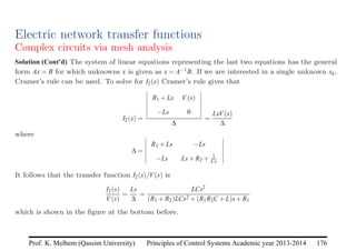
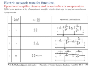
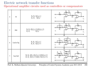
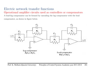
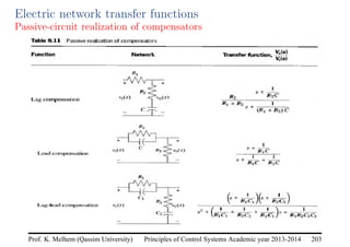
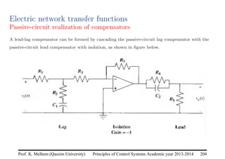
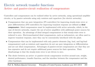
The document discusses the modeling of electrical and mechanical systems using transfer functions and state-space representations, focusing on the application of Kirchhoff's laws. It explains the concepts of impedance and admittance, and how they facilitate the simplification of circuit analysis through mesh and nodal analysis techniques. Various examples illustrate the derivation of transfer functions for simple and complex circuits, emphasizing the systematic approach to solving electrical networks.
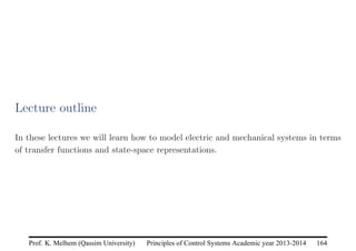

![Principles of Control Systems Academic year 2013-2014 171
Prof. K. Melhem (Qassim University)
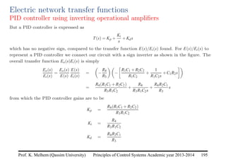
Electric network transfer functions
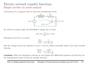
Simple circuits via mesh analysis
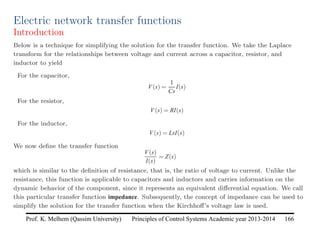
The Laplace transform of the loop differential equation, assuming zero initial conditions, is
(Ls+R+
1
Cs
)I(s) = V(s)
which is in the form
[Sum of impedances] I(s) = [Sum of applied voltages]
The last form suggests the circuit shown below
in which we add impedances in series as we add resistors in series. We notice that the circuit above
could have been obtained immediately from the original network circuit simply by replacing each
component with its impedance. We call this altered circuit the transformed circuit.](https://image.slidesharecdn.com/lectures1215modelingofelectricalan-240517172255-5a158b43/85/Lectures_12_15_Modeling_of_Electrical_an-pdf-9-320.jpg)
![Principles of Control Systems Academic year 2013-2014 180
Prof. K. Melhem (Qassim University)
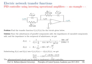
Electric network transfer functions
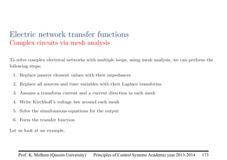
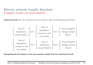
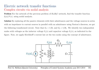
Simple circuits via nodal analysis
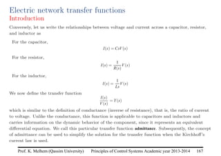
Solution Notice that the last equation can be rewritten as
1
R+Ls
+Cs
VC(s) =
1
R+Ls
V(s)
which is in the form
[Sum of admittances connected to the node] VC(s) = [Sum of applied currents at the node]
This suggests the following transformed circuit given now with current source and admittances
rather than voltage source and impedances.
1/(R+Ls)V(s) 1/(R+Ls)
Cs VC(s)](https://image.slidesharecdn.com/lectures1215modelingofelectricalan-240517172255-5a158b43/85/Lectures_12_15_Modeling_of_Electrical_an-pdf-18-320.jpg)
![Principles of Control Systems Academic year 2013-2014 183
Prof. K. Melhem (Qassim University)
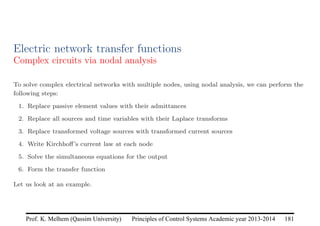
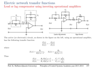
Electric network transfer functions
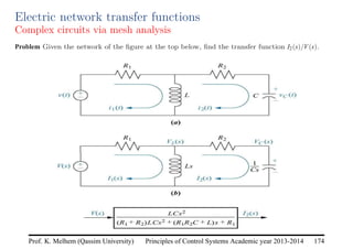
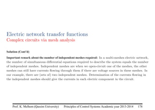
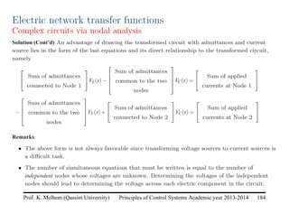
Complex circuits via nodal analysis
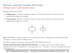
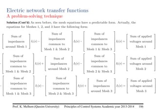
Solution (Cont’d)
Summing currents at the node VL(s) yields
G1[VL(s)−V(s)]+
1
Ls
VL(s)+G2[VL(s)−VC(s)] = 0
Summing currents at the node VC(s) yields
CsVC(s)+G2[VC(s)−VL(s)] = 0
Combining terms, the last two equations can be rewritten as simultaneous equations in VL(s) and
VC(s) as
G1 +G2 +
1
Ls
VL(s)−G2VC(s) = V(s)G1
−G2VL(s)+(G2 +Cs)VC(s) = 0
Solving for the transfer function VC(s)/V(s) yields
VC(s)
V(s)
=
G1G2
C s
(G1 +G2)s2 + G1G2L+C
LC s+ G2
LC](https://image.slidesharecdn.com/lectures1215modelingofelectricalan-240517172255-5a158b43/85/Lectures_12_15_Modeling_of_Electrical_an-pdf-21-320.jpg)
![Principles of Control Systems Academic year 2013-2014 190
Prof. K. Melhem (Qassim University)
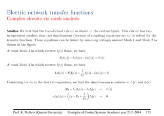
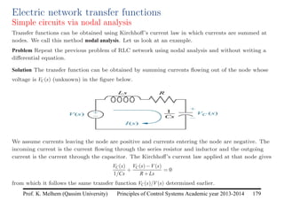
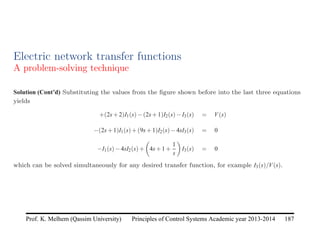
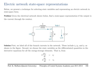
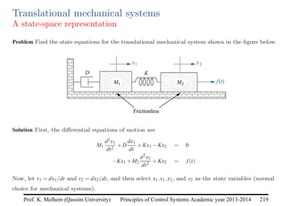
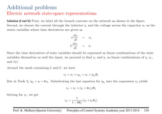
Electric network state-space representations
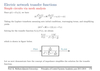
Or
dvC
dt
= −
1
RC
vC +
1
C
iL
diL
dt
= −
1
L
vC +
1
L
v(t)
Since the output is chosen as iR(t), the output equation is
iR =
1
R
vC
which is a linear combination of state variable vC.
Finally, the state-space representation in matrix form is
v̇C
i̇L
=
−1/(RC) 1/C
−1/L 0
vC
iL
+
0
1/L
v
iR = [1/R 0]
vC
iL
](https://image.slidesharecdn.com/lectures1215modelingofelectricalan-240517172255-5a158b43/85/Lectures_12_15_Modeling_of_Electrical_an-pdf-28-320.jpg)
![Principles of Control Systems Academic year 2013-2014 210
Prof. K. Melhem (Qassim University)
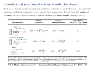
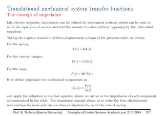
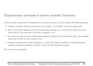
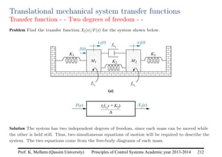
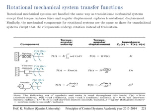
Translational mechanical system transfer functions
Transfer function - - One degree of freedom - -
Solution We now write the differential equation of motion using Newton’s second law to sum to zero
the different forces acting on the mass and to yield
M
d2x(t)
dt2
+ fv
dx(t)
dt
+Kx(t) = f(t)
Taking the Laplace transform, assuming zero initial conditions,
Ms2
X(s)+ fvsX(s)+KX(s) = F(s) or (Ms2
+ fvs+K)X(s) = F(s)
Solving for the transfer function yields
G(s) =
X(s)
F(s)
=
1
Ms2 + fvs+K
Using the concept of impedance, we notice that the Laplace-transformed equation of motion is of
the form
[Sum of impedances connected to the motion at x] X(s) = [Sum of applied forces at x]](https://image.slidesharecdn.com/lectures1215modelingofelectricalan-240517172255-5a158b43/85/Lectures_12_15_Modeling_of_Electrical_an-pdf-48-320.jpg)
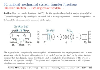
![Principles of Control Systems Academic year 2013-2014 218
Prof. K. Melhem (Qassim University)
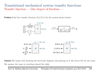
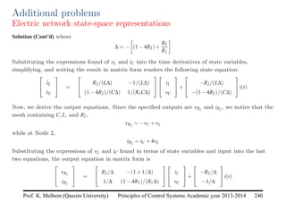
Translational mechanical system transfer functions
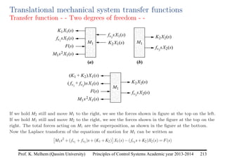
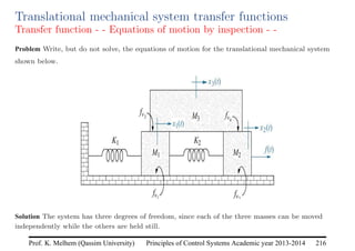
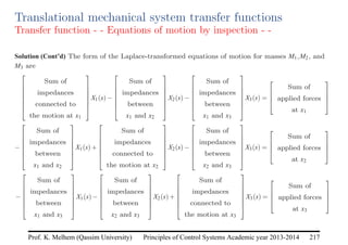
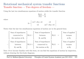
Transfer function - - Equations of motion by inspection - -
Solution (Cont’d) M1 has two springs, two viscous dampers, and mass associated with its motion.
There is one spring between M1 and M2, and one viscous damper between M1 and M3. Thus, the
equation of motion for M1 is
[M1s2
+( fv1 + fv3 )s+(K1 +K2)]X1(s)−K2X2(s)− fv3 sX3(s) = 0
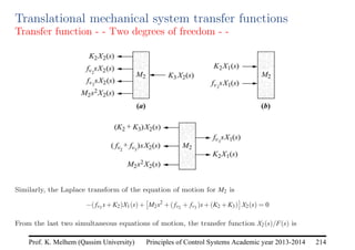
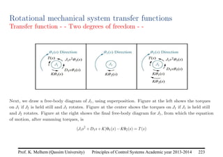
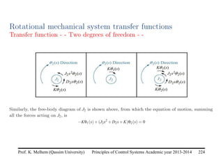
Similarly, the equations of motion for M2 and M3 are
−K2X1(s)+[M2s2
+( fv2 + fv4 )s+K2]X2(s)− fv4 sX3(s) = F(s)
− fv3 sX1(s)− fv4 sX2(s)+[M3s2
+( fv3 + fv4 )s]X3(s) = 0
Note: We can solve the last equations for any displacements X1(s),X2(s), or X3(s), or transfer
function.](https://image.slidesharecdn.com/lectures1215modelingofelectricalan-240517172255-5a158b43/85/Lectures_12_15_Modeling_of_Electrical_an-pdf-56-320.jpg)
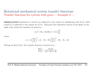
![Principles of Control Systems Academic year 2013-2014 239
Prof. K. Melhem (Qassim University)
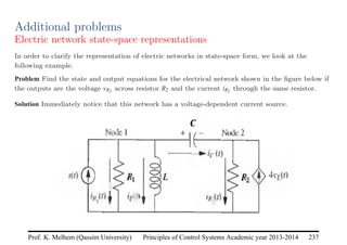
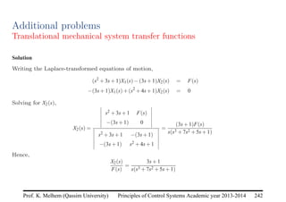
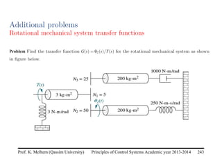
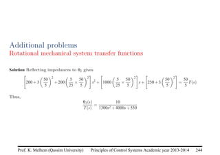
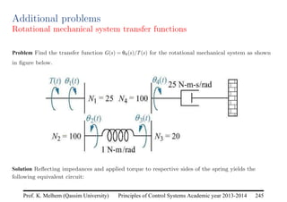
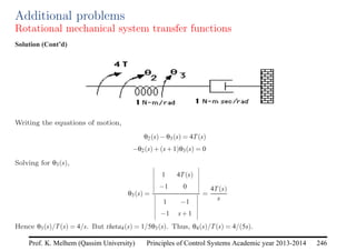
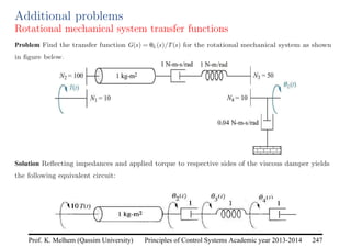
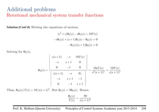
Additional problems
Electric network state-space representations
Solution (Cont’d) Now, we need to find iC in terms of state variables and input. Thus, at Node 1 we
can write the sum of the currents as
iC = i−iR1 −iL
= i−
vR1
R1
−iL
= i−
vL
R1
−iL
Last equation are simultaneous relating vL and iC in terms of the state variables iL and vC, as well
the input i(t). These equations can be rewritten as
(1−4R2)vL −R2iC = vC
−
1
R1
vL −iC = iL −i(t)
Solving simultaneously for vL and iC, using Cramer’s rule, yields
vL =
1
∆
[R2iL −vC −R2i(t)]
and
iC =
1
∆
[(1−4R2)iL +
1
R1
vC −(1−4R2)i(t)]](https://image.slidesharecdn.com/lectures1215modelingofelectricalan-240517172255-5a158b43/85/Lectures_12_15_Modeling_of_Electrical_an-pdf-77-320.jpg)


![[Deck] What's New in Spark-Iceberg Integration via DSV2.pptx](https://cdn.slidesharecdn.com/ss_thumbnails/deckwhatsnewinspark-icebergintegrationviadsv2-260210005337-25955b12-thumbnail.jpg?width=640&height=640&fit=bounds)


