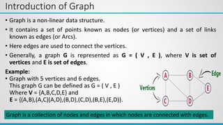
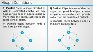
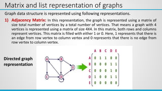
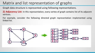
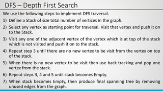
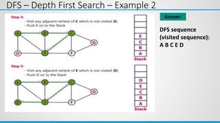
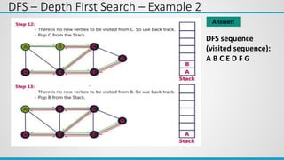
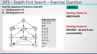
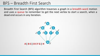
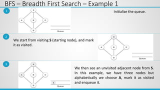
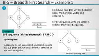
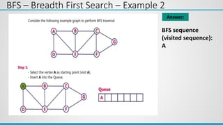
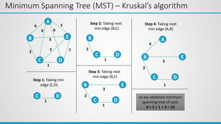
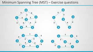
This document provides an overview of the topics covered in Unit 5, which include graphs, hashing, and collision resolution techniques. It defines graphs and their components such as vertices, edges, directed and undirected graphs. It also discusses different graph representations like adjacency matrix and adjacency list. Elementary graph operations like breadth-first search and depth-first search are explained along with examples. Hashing functions and collision resolution are also introduced.


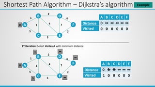
![Shortest Path Algorithm – Dijkstra’s algorithm Example
A
B
C
D
E
F
1
1
5
2
4 7
6
2
0
2nd Iteration: Select Vertex B with minimum distance
1
2
Cost of going to C via B = dist[B] + cost[B][C] = 1 + 1 = 2
Cost of going to D via B = dist[B] + cost[B][D] = 1 + 2 = 3
Cost of going to E via B = dist[B] + cost[B][E] = 1 + 4 = 5
Cost of going to F via B = dist[B] + cost[B][F] = 1 + ∞ = ∞
A B C D E F
0 1 5 ∞ ∞ ∞
1 0 0 0 0 0
Distance
Visited
3
5
∞
A B C D E F
0 1 2 3 5 ∞
0 0 0
Distance
Visited 1 1 0
5](https://image.slidesharecdn.com/unit-6graph-240227125144-d21bd2d3/85/Unit-6-Graph-ppsx-ppt-52-320.jpg)
![Shortest Path Algorithm – Dijkstra’s algorithm Example
3rd Iteration: Select Vertex C via B with minimum distance
A B C D E F
0 1 2 3 5 ∞
1 1 0 0 0 0
Distance
Visited
A
B
C
D
E
F
1
1
5
2
4 7
6
2
0
1 3
2 5
∞
Cost of going to D via C = dist[C] + cost[C][D] = 2 + ∞ = ∞
Cost of going to E via C = dist[C] + cost[C][E] = 2 + 5 = 7
Cost of going to F via C = dist[C] + cost[C][F] = 2 + ∞ = ∞
A B C D E F
0 1 2 3 5 ∞
0 0 0
Distance
Visited 1 1 1
5](https://image.slidesharecdn.com/unit-6graph-240227125144-d21bd2d3/85/Unit-6-Graph-ppsx-ppt-53-320.jpg)
![Shortest Path Algorithm – Dijkstra’s algorithm Example
4th Iteration: Select Vertex D via path A - B with minimum distance
A B C D E F
0 1 2 3 5 ∞
1 1 1 0 0 0
Distance
Visited
A
B
C
D
E
F
1
1
5
2
4 7
6
2
1 3
2 5
9
Cost of going to E via D = dist[D] + cost[D][E] = 3 + 7 = 10
Cost of going to F via D = dist[D] + cost[D][F] = 3 + 6 = 9
A B C D E F
0 1 2 3 5 9
1 0 0
Distance
Visited 1 1 1
5](https://image.slidesharecdn.com/unit-6graph-240227125144-d21bd2d3/85/Unit-6-Graph-ppsx-ppt-54-320.jpg)
![Shortest Path Algorithm – Dijkstra’s algorithm Example
4th Iteration: Select Vertex E via path A – B – E with minimum distance
A B C D E F
0 1 2 3 5 9
1 1 1 1 0 0
Distance
Visited
A
B
C
D
E
F
1
1
5
2
4 7
6
2
1 3
2 5
7
Cost of going to F via E = dist[E] + cost[E][F] = 5 + 2 = 7
A B C D E F
0 1 2 3 5 7
1 1 0
Distance
Visited 1 1 1
Shortest Path from A to F is
A B E F = 7](https://image.slidesharecdn.com/unit-6graph-240227125144-d21bd2d3/85/Unit-6-Graph-ppsx-ppt-55-320.jpg)