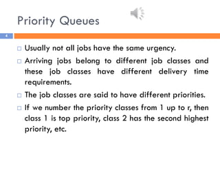
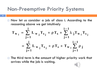
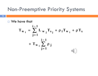
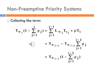
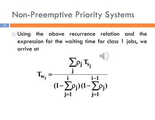
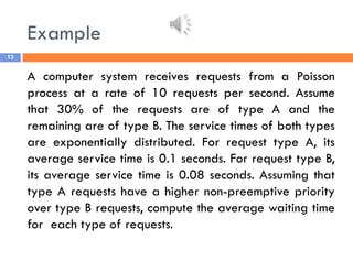
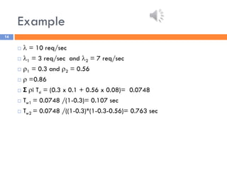
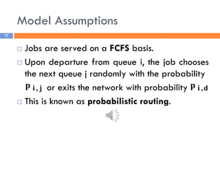
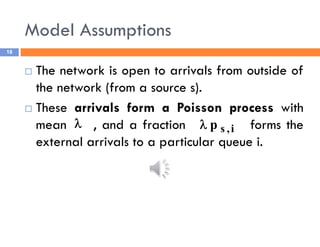
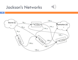
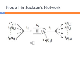
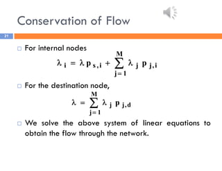
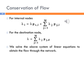
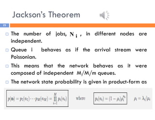
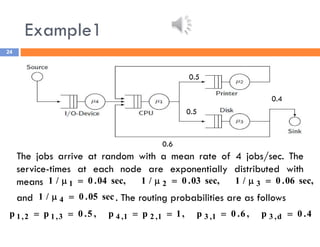
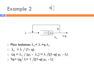
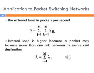
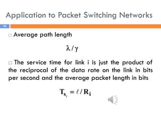
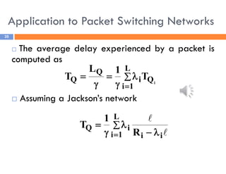
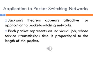
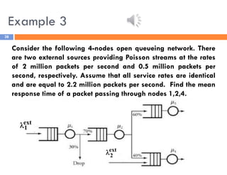
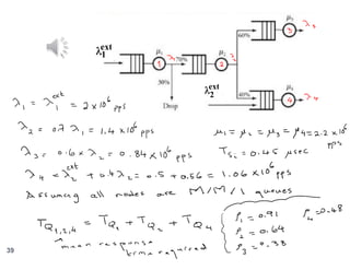
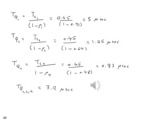
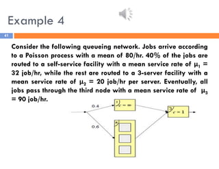
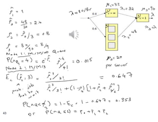
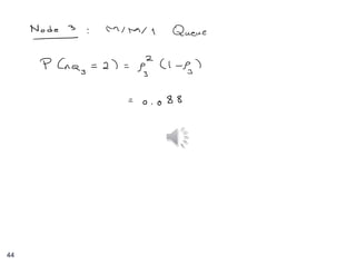
‫اﻟرﺣﯾم‬ ‫اﻟرﺣﻣن‬ ‫ﷲ‬ ‫ﺑﺳم‬
‫أﻧﯾب‬ ‫إﻟﯾﮫ‬ ‫و‬ ‫ﺗوﻛﻠت‬ ‫ﻋﻠﯾﮫ‬ ‫ﺑﺎ‬ ‫إﻻ‬ ‫ﺗوﻓﯾﻘﻲ‬ ‫ﻣﺎ‬ ‫و‬
Outline
2
 Priority queues
 Jackson’s networks
 Assumptions
 Theorem
 Application
 Closed queueing networks
 Gordon-Newell network model
 Mean-Value-Analysis (MVA) algorithm
 Application
• Model assumptions
• Mean waiting time expressions for
different classes
Priority Queues
Priority Queues
4
 Usually not all jobs have the same urgency.
 Arriving jobs belong to different job classes and
these job classes have different delivery time
requirements.
 The job classes are said to have different priorities.
 If we number the priority classes from 1 up to r, then
class 1 is top priority, class 2 has the second highest
priority, etc.
Priority Queues
5
 There are two variants of the priority rule.
 In the first one a job that has started cannot be
interrupted; in the second one the processing of a
job can be interrupted by newly arrived jobs of
higher priority classes.
 If all higher priority jobs are served, the servicing
of the job is resumed where it was preempted, i.e.,
no work is lost.
 The first type of priority is called non-preemptive,
the second type is called preemptive-resume.
Non-Preemptive Priority Systems
6
 Consider an M/M/1 queueing system with non-
preemptive priorities.
 Let us first look at a job of class 1. This job has to
wait for jobs of its own class that arrived before,
and also for the job (if any) on the machine.
 Then,
i
i
1
1
1
s
r
1
i
i
s
r
1
i
i
s
r
1
i
i
s
w
w
T
T
,
T
T
L
T















Non-Preemptive Priority Systems
7
 Using Little’s law and simplifying:
1
j
s
j
1
s
w
s
w
1
s
s
w
1
s
s
w
w
1
T
1
T
T
T
T
T
T
T
T
T
L
T
j
1
1
1
1
1
1
1




















Non-Preemptive Priority Systems
8
 For the job classes i = 2, ..., r, the situation is more
complicated. Apart from the amount of work found
upon arrival that a job has to wait for, a job also
has to wait for higher priority jobs that arrive later
while it is waiting in the queue.
Non-Preemptive Priority Systems
9
 Now let us consider a job of class i. According to the
reasoning above we get intuitively
 The third term is the amount of higher priority work that
arrives while the job is waiting.




















1
i
1
j
j
w
s
i
1
j
s
w
s
1
i
1
j
w
j
s
i
1
j
s
w
w
i
j
j
j
i
j
j
i
T
T
T
L
T
T
T
T
L
T
Non-Preemptive Priority Systems
10
 We have that













1
i
1
j
j
w
s
w
i
1
i
1
j
s
w
w
i
i
j
j
i
T
T
T
T
L
T
Non-Preemptive Priority Systems
11
 Collecting like terms
)
1
(
T
T
T
T
T
L
)
1
(
T
2
i
1
j
j
w
2
i
1
j
j
w
w
s
1
i
1
j
s
w
i
1
j
j
w
1
i
1
i
1
i
j
j
i

























Non-Preemptive Priority Systems
12
 Using the above recurrence relation and the
expression for the waiting time for class 1 jobs, we
arrive at
)
1
(
)
1
(
T
T
1
i
1
j
j
i
1
j
j
j
s
j
w
j
i












Example
13
A computer system receives requests from a Poisson
process at a rate of 10 requests per second. Assume
that 30% of the requests are of type A and the
remaining are of type B. The service times of both types
are exponentially distributed. For request type A, its
average service time is 0.1 seconds. For request type B,
its average service time is 0.08 seconds. Assuming that
type A requests have a higher non-preemptive priority
over type B requests, compute the average waiting time
for each type of requests.
Example
14
  = 10 req/sec
 1 = 3 req/sec and 2 = 7 req/sec
 1 = 0.3 and 2 = 0.56
  =0.86
 i Tsi = (0.3 x 0.1 + 0.56 x 0.08)= 0.0748
 Tw1 = 0.0748 /(1-0.3)= 0.107 sec
 Tw2 = 0.0748 /((1-0.3)*(1-0.3-0.56)= 0.763 sec
• Model assumptions
• Jackson’s theorem
• Applications
Jackson’s Networks
Model Assumptions
16
 A Jackson network is a particular type of open
network.
 It consists of ‘M’ nodes or service centers.
 Each service center consists of a fixed number
of servers and the service time at each center
is exponentially distributed.
 In each queue, the service time of the job is
drawn independent of the service times in
other queues.
Model Assumptions
17
 Jobs are served on a FCFS basis.
 Upon departure from queue i, the job chooses
the next queue j randomly with the probability
or exits the network with probability
 This is known as probabilistic routing.
j
,
i
p d
,
i
p
Model Assumptions
18
 The network is open to arrivals from outside of
the network (from a source s).
 These arrivals form a Poisson process with
mean , and a fraction forms the
external arrivals to a particular queue i.
 i
,
s
p

Jackson’s Networks
19
Source (s)
Destination (d)
Node i in Jackson’s Network
20
Conservation of Flow
21
 For internal nodes
 For the destination node,
 We solve the above system of linear equations to
obtain the flow through the network.







M
1
j
i
,
j
j
i
,
s
i p
p





M
1
j
d
,
j
j p
Conservation of Flow
22
 For internal nodes
 For the destination node,
 We solve the above system of linear equations to
obtain the flow through the network.







M
1
j
i
,
j
j
i
,
s
i p
p





M
1
j
d
,
j
j p
Jackson’s Theorem
23
 The number of jobs, , in different nodes are
independent.
 Queue i behaves as if the arrival stream were
Poissonian.
 This means that the network behaves as it were
composed of independent M/M/m queues.
 The network state probability is given in product-form as
i
N
Example1
24
The jobs arrive at random with a mean rate of 4 jobs/sec. The
service-times at each node are exponentially distributed with
means
and . The routing probabilities are as follows
sec,
06
.
0
/
1
sec,
03
.
0
/
1
sec,
04
.
0
/
1 3
2
1 





sec
05
.
0
/
1 4 

4
.
0
p
,
6
.
0
p
,
1
p
p
,
5
.
0
p
p d
,
3
1
,
3
1
,
2
1
,
4
3
,
1
2
,
1 





0.5
0.5
0.4
0.6
Example 1 (continued)
25
 What is the steady state probability of the network
state (3,2,4,1)?
 Compute the mean number of jobs in each queue
 Compute the mean overall response time (or the mean
time spent by a job in the system).
Example 1
26
  = 4 jobs/sec
 Ts1 = 0.04 sec, Ts2 = 0.03 sec, Ts3 = 0.06 sec, Ts4 = 0.05 sec
 Flow balance
 at node 1 (CPU): 1= 4 + 2 +0.6 3
 at node 2: 2 = 0.5 1
 at node 3: 3 = 0.5 1
 Substitute back in 1st eqn: (1- 0.5 – 0.3) 1 = 4
 1 = 20 job/sec, 2 = 3 = 10 jobs/sec
 1 = 0.8, 2 = 0.3, 3 = 0.6, 4 = 0.2
Example 1
27
 Prob. of joint state (3,2,4,1) is 0.0000535
 Lq1= 4 , Lq2 = 0.43, Lq3 =1.5, Lq4 =0.25
 Tq= (Lq1+Lq2+Lq3+Lq4) /  = 1.545 sec
Example 2
28
Consider a switching facility that transmits messages to a required destination. A
NACK is sent by the destination when a packet has not been properly received.
If so, the packet in error is retransmitted as soon as the NACK is received. Assume
the time to send a message and the time to receive a NACK are both
independent and identically distributed exponential random variables. Assume
that packets arrive at the switch according to a Poisson process with rate λ. Let q
be the probability that a message is received incorrectly. This system can be
modeled by the open queueing network shown in figure. Determine the following:
(i) the mean number of messages in the system. (ii) the mean time-in-system.
Example 2
29
 Flow balance: 1=  +q 1
 1 =  / (1- q)
 Lq = 1 / (1 - 1) =  /((1-q) 1 - )
 Tq= Lq/ = 1 /((1-q) 1 - )
1
Application to Packet Switching Networks
30
 A packet-switching network is a digital
communications network that groups all transmitted
data into suitably sized blocks called packets.
 The network over which packets are transmitted is a
shared network which routes each packet
independently of all others and allocates transmission
resources as needed.
Application to Packet Switching Networks
31
 The principal goals of packet switching are to
 optimize utilization of available link capacity
 minimize response times
 increase robustness of communication
Application to Packet Switching Networks
32
 When traversing network adapters, switches and
other network nodes, packets are buffered and
queued, resulting in variable delay and throughput,
depending on the traffic load in the network.
Application to Packet Switching Networks
33
 The external load in packets per second
 Internal load is higher because a packet may
traverse more than one link between its source and
destination
 
 



M
1
j
M
1
k
jk





M
1
i
i
Application to Packet Switching Networks
34
 Average path length
 The service time for link i is just the product of
the reciprocal of the data rate on the link in bits
per second and the average packet length in bits

 /
i
s R
/
T i


Application to Packet Switching Networks
35
 The average delay experienced by a packet is
computed as
 Assuming a Jackson’s network
i
Q
L
1
i
i
Q
Q T
1
L
T 








i
i
L
1
i
i
Q
R
1
T




 

Application to Packet Switching Networks
36
 Jackson’s theorem appears attractive for
application to packet-switching networks.
 Each packet represents an individual job, whose
service (transmission) time is proportional to the
length of the packet.
Application to Packet Switching Networks
37
 The flaw in applying Jackson’s theorem is the
assumption that the service-time distributions at
different nodes are independent.
 In fact, the service-times at different nodes are
proportional.
 However, Kleinrock has demonstrated that still
Jackson’s theorem provides a quite good
approximation.
Example 3
38
Consider the following 4-nodes open queueing network. There
are two external sources providing Poisson streams at the rates
of 2 million packets per second and 0.5 million packets per
second, respectively. Assume that all service rates are identical
and are equal to 2.2 million packets per second. Find the mean
response time of a packet passing through nodes 1,2,4.
ext
2

ext
1

39
ext
2

ext
1

40
Example 4
41
Consider the following queueing network. Jobs arrive according
to a Poisson process with a mean of 80/hr. 40% of the jobs are
routed to a self-service facility with a mean service rate of μ1 =
32 job/hr, while the rest are routed to a 3-server facility with a
mean service rate of μ2 = 20 job/hr per server. Eventually, all
jobs pass through the third node with a mean service rate of μ3
= 90 job/hr.
Example 4
42
Assuming exponentially distributed service times,
determine the probability that:
i) there are 4 jobs at node 1.
ii) a job does not have to wait at node 2.
iii) there are 2 jobs at node 3.
(Hint: All nodes behave as independent M/M/c
queues).
43
44
45
THANK YOU

Lecture 8performanceevaluationnperfo.pdf

  • 1.
    ‫اﻟرﺣﯾم‬ ‫اﻟرﺣﻣن‬ ‫ﷲ‬‫ﺑﺳم‬ ‫أﻧﯾب‬ ‫إﻟﯾﮫ‬ ‫و‬ ‫ﺗوﻛﻠت‬ ‫ﻋﻠﯾﮫ‬ ‫ﺑﺎ‬ ‫إﻻ‬ ‫ﺗوﻓﯾﻘﻲ‬ ‫ﻣﺎ‬ ‫و‬
  • 2.
    Outline 2  Priority queues Jackson’s networks  Assumptions  Theorem  Application  Closed queueing networks  Gordon-Newell network model  Mean-Value-Analysis (MVA) algorithm  Application
  • 3.
    • Model assumptions •Mean waiting time expressions for different classes Priority Queues
  • 4.
    Priority Queues 4  Usuallynot all jobs have the same urgency.  Arriving jobs belong to different job classes and these job classes have different delivery time requirements.  The job classes are said to have different priorities.  If we number the priority classes from 1 up to r, then class 1 is top priority, class 2 has the second highest priority, etc.
  • 5.
    Priority Queues 5  Thereare two variants of the priority rule.  In the first one a job that has started cannot be interrupted; in the second one the processing of a job can be interrupted by newly arrived jobs of higher priority classes.  If all higher priority jobs are served, the servicing of the job is resumed where it was preempted, i.e., no work is lost.  The first type of priority is called non-preemptive, the second type is called preemptive-resume.
  • 6.
    Non-Preemptive Priority Systems 6 Consider an M/M/1 queueing system with non- preemptive priorities.  Let us first look at a job of class 1. This job has to wait for jobs of its own class that arrived before, and also for the job (if any) on the machine.  Then, i i 1 1 1 s r 1 i i s r 1 i i s r 1 i i s w w T T , T T L T               
  • 7.
    Non-Preemptive Priority Systems 7 Using Little’s law and simplifying: 1 j s j 1 s w s w 1 s s w 1 s s w w 1 T 1 T T T T T T T T T L T j 1 1 1 1 1 1 1                    
  • 8.
    Non-Preemptive Priority Systems 8 For the job classes i = 2, ..., r, the situation is more complicated. Apart from the amount of work found upon arrival that a job has to wait for, a job also has to wait for higher priority jobs that arrive later while it is waiting in the queue.
  • 9.
    Non-Preemptive Priority Systems 9 Now let us consider a job of class i. According to the reasoning above we get intuitively  The third term is the amount of higher priority work that arrives while the job is waiting.                     1 i 1 j j w s i 1 j s w s 1 i 1 j w j s i 1 j s w w i j j j i j j i T T T L T T T T L T
  • 10.
    Non-Preemptive Priority Systems 10 We have that              1 i 1 j j w s w i 1 i 1 j s w w i i j j i T T T T L T
  • 11.
    Non-Preemptive Priority Systems 11 Collecting like terms ) 1 ( T T T T T L ) 1 ( T 2 i 1 j j w 2 i 1 j j w w s 1 i 1 j s w i 1 j j w 1 i 1 i 1 i j j i                         
  • 12.
    Non-Preemptive Priority Systems 12 Using the above recurrence relation and the expression for the waiting time for class 1 jobs, we arrive at ) 1 ( ) 1 ( T T 1 i 1 j j i 1 j j j s j w j i            
  • 13.
    Example 13 A computer systemreceives requests from a Poisson process at a rate of 10 requests per second. Assume that 30% of the requests are of type A and the remaining are of type B. The service times of both types are exponentially distributed. For request type A, its average service time is 0.1 seconds. For request type B, its average service time is 0.08 seconds. Assuming that type A requests have a higher non-preemptive priority over type B requests, compute the average waiting time for each type of requests.
  • 14.
    Example 14   =10 req/sec  1 = 3 req/sec and 2 = 7 req/sec  1 = 0.3 and 2 = 0.56   =0.86  i Tsi = (0.3 x 0.1 + 0.56 x 0.08)= 0.0748  Tw1 = 0.0748 /(1-0.3)= 0.107 sec  Tw2 = 0.0748 /((1-0.3)*(1-0.3-0.56)= 0.763 sec
  • 15.
    • Model assumptions •Jackson’s theorem • Applications Jackson’s Networks
  • 16.
    Model Assumptions 16  AJackson network is a particular type of open network.  It consists of ‘M’ nodes or service centers.  Each service center consists of a fixed number of servers and the service time at each center is exponentially distributed.  In each queue, the service time of the job is drawn independent of the service times in other queues.
  • 17.
    Model Assumptions 17  Jobsare served on a FCFS basis.  Upon departure from queue i, the job chooses the next queue j randomly with the probability or exits the network with probability  This is known as probabilistic routing. j , i p d , i p
  • 18.
    Model Assumptions 18  Thenetwork is open to arrivals from outside of the network (from a source s).  These arrivals form a Poisson process with mean , and a fraction forms the external arrivals to a particular queue i.  i , s p 
  • 19.
  • 20.
    Node i inJackson’s Network 20
  • 21.
    Conservation of Flow 21 For internal nodes  For the destination node,  We solve the above system of linear equations to obtain the flow through the network.        M 1 j i , j j i , s i p p      M 1 j d , j j p
  • 22.
    Conservation of Flow 22 For internal nodes  For the destination node,  We solve the above system of linear equations to obtain the flow through the network.        M 1 j i , j j i , s i p p      M 1 j d , j j p
  • 23.
    Jackson’s Theorem 23  Thenumber of jobs, , in different nodes are independent.  Queue i behaves as if the arrival stream were Poissonian.  This means that the network behaves as it were composed of independent M/M/m queues.  The network state probability is given in product-form as i N
  • 24.
    Example1 24 The jobs arriveat random with a mean rate of 4 jobs/sec. The service-times at each node are exponentially distributed with means and . The routing probabilities are as follows sec, 06 . 0 / 1 sec, 03 . 0 / 1 sec, 04 . 0 / 1 3 2 1       sec 05 . 0 / 1 4   4 . 0 p , 6 . 0 p , 1 p p , 5 . 0 p p d , 3 1 , 3 1 , 2 1 , 4 3 , 1 2 , 1       0.5 0.5 0.4 0.6
  • 25.
    Example 1 (continued) 25 What is the steady state probability of the network state (3,2,4,1)?  Compute the mean number of jobs in each queue  Compute the mean overall response time (or the mean time spent by a job in the system).
  • 26.
    Example 1 26  = 4 jobs/sec  Ts1 = 0.04 sec, Ts2 = 0.03 sec, Ts3 = 0.06 sec, Ts4 = 0.05 sec  Flow balance  at node 1 (CPU): 1= 4 + 2 +0.6 3  at node 2: 2 = 0.5 1  at node 3: 3 = 0.5 1  Substitute back in 1st eqn: (1- 0.5 – 0.3) 1 = 4  1 = 20 job/sec, 2 = 3 = 10 jobs/sec  1 = 0.8, 2 = 0.3, 3 = 0.6, 4 = 0.2
  • 27.
    Example 1 27  Prob.of joint state (3,2,4,1) is 0.0000535  Lq1= 4 , Lq2 = 0.43, Lq3 =1.5, Lq4 =0.25  Tq= (Lq1+Lq2+Lq3+Lq4) /  = 1.545 sec
  • 28.
    Example 2 28 Consider aswitching facility that transmits messages to a required destination. A NACK is sent by the destination when a packet has not been properly received. If so, the packet in error is retransmitted as soon as the NACK is received. Assume the time to send a message and the time to receive a NACK are both independent and identically distributed exponential random variables. Assume that packets arrive at the switch according to a Poisson process with rate λ. Let q be the probability that a message is received incorrectly. This system can be modeled by the open queueing network shown in figure. Determine the following: (i) the mean number of messages in the system. (ii) the mean time-in-system.
  • 29.
    Example 2 29  Flowbalance: 1=  +q 1  1 =  / (1- q)  Lq = 1 / (1 - 1) =  /((1-q) 1 - )  Tq= Lq/ = 1 /((1-q) 1 - ) 1
  • 30.
    Application to PacketSwitching Networks 30  A packet-switching network is a digital communications network that groups all transmitted data into suitably sized blocks called packets.  The network over which packets are transmitted is a shared network which routes each packet independently of all others and allocates transmission resources as needed.
  • 31.
    Application to PacketSwitching Networks 31  The principal goals of packet switching are to  optimize utilization of available link capacity  minimize response times  increase robustness of communication
  • 32.
    Application to PacketSwitching Networks 32  When traversing network adapters, switches and other network nodes, packets are buffered and queued, resulting in variable delay and throughput, depending on the traffic load in the network.
  • 33.
    Application to PacketSwitching Networks 33  The external load in packets per second  Internal load is higher because a packet may traverse more than one link between its source and destination        M 1 j M 1 k jk      M 1 i i
  • 34.
    Application to PacketSwitching Networks 34  Average path length  The service time for link i is just the product of the reciprocal of the data rate on the link in bits per second and the average packet length in bits   / i s R / T i  
  • 35.
    Application to PacketSwitching Networks 35  The average delay experienced by a packet is computed as  Assuming a Jackson’s network i Q L 1 i i Q Q T 1 L T          i i L 1 i i Q R 1 T       
  • 36.
    Application to PacketSwitching Networks 36  Jackson’s theorem appears attractive for application to packet-switching networks.  Each packet represents an individual job, whose service (transmission) time is proportional to the length of the packet.
  • 37.
    Application to PacketSwitching Networks 37  The flaw in applying Jackson’s theorem is the assumption that the service-time distributions at different nodes are independent.  In fact, the service-times at different nodes are proportional.  However, Kleinrock has demonstrated that still Jackson’s theorem provides a quite good approximation.
  • 38.
    Example 3 38 Consider thefollowing 4-nodes open queueing network. There are two external sources providing Poisson streams at the rates of 2 million packets per second and 0.5 million packets per second, respectively. Assume that all service rates are identical and are equal to 2.2 million packets per second. Find the mean response time of a packet passing through nodes 1,2,4. ext 2  ext 1 
  • 39.
  • 40.
  • 41.
    Example 4 41 Consider thefollowing queueing network. Jobs arrive according to a Poisson process with a mean of 80/hr. 40% of the jobs are routed to a self-service facility with a mean service rate of μ1 = 32 job/hr, while the rest are routed to a 3-server facility with a mean service rate of μ2 = 20 job/hr per server. Eventually, all jobs pass through the third node with a mean service rate of μ3 = 90 job/hr.
  • 42.
    Example 4 42 Assuming exponentiallydistributed service times, determine the probability that: i) there are 4 jobs at node 1. ii) a job does not have to wait at node 2. iii) there are 2 jobs at node 3. (Hint: All nodes behave as independent M/M/c queues).
  • 43.
  • 44.
  • 45.