This document provides a summary of the book "Queueing Modelling Fundamentals with Applications in Communication Networks" by Ng Chee-Hock and Soong Boon-Hee. It is the second edition of this book published by John Wiley & Sons Ltd. The book covers fundamental concepts in queueing theory and its applications in modeling communication networks. It includes chapters on probability theory, Markov processes, single and multi-server queueing systems, semi-Markovian queues, open and closed queueing networks, and flow control mechanisms.


![2 PRELIMINARIES
importance of probability theory in queueing analysis cannot be over-
emphasized. It plays a central role as that of the limiting concept to calculus.
The development of probability theory is closely related to describing ran-
domly occurring events and has its roots in predicting the random outcome
of playing games. We shall begin by defining the notion of an event and the
sample space of a mathematical experiment which is supposed to mirror a
real-life phenomenon.
1.1.1 Sample Spaces and Axioms of Probability
A sample space (Ω) of a random experiment is a collection of all the mutually
exclusive and exhaustive simple outcomes of that experiment. A particular
simple outcome (w) of an experiment is often referred to as a sample point. An
event (E) is simply a subset of Ω and it contains a set of sample points that
satisfy certain common criteria. For example, an event could be the even
numbers in the toss of a dice and it contains those sample points {[2], [4], [6]}.
We indicate that the outcome w is a sample point of an event E by writing
{w ∈ E}. If an event E contains no sample points, then it is a null event and
we write E = ∅. Two events E and F are said to be mutually exclusive if they
have no sample points in common, or in other words the intersection of events
E and F is a null event, i.e. E ∩ F = ∅.
There are several notions of probability. One of the classic definitions is
based on the relative frequency approach in which the probability of an event
E is the limiting value of the proportion of times that E was observed.
That is
P E
N
N
N
E
( ) =
→∞
lim (1.1)
where NE is the number of times event E was observed and N is the total
number of observations. Another one is the so-called axiomatic approach
where the probability of an event E is taken to be a real-value function
defined on the family of events of a sample space and satisfies the following
conditions:
Axioms of probability
(i) 0 ≤ P(E) ≤ 1 for any event in that experiment
(ii) P(Ω) = 1
(iii) If E and F are mutually exclusive events, i.e. E ∈ F = ∅, then P(E ∪ F)
= P(E) + P(F)](https://image.slidesharecdn.com/qtts-230925120453-047b3b23/85/QTTS-pdf-25-320.jpg)
![8 PRELIMINARIES
A concept closely related to a random variable is its cumulative probabil-
ity distribution function, or just distribution function (PDF). It is defined
as
F x P X x
P X x
X ( ) [ ]
[ : ( ) ]
≡ ≤
= ≤
ω ω (1.7)
For simplicity, we usually drop the subscript X when the random variable
of the function referred to is clear in the context. Students should note that
a distribution function completely describes a random variable, as all param-
eters of interest can be derived from it. It can be shown from the basic
axioms of probability that a distribution function possesses the following
properties:
Proposition 1.2
(i) F is a non-negative and non-decreasing function, i.e. if x1 ≤ x2 then
F(x1) ≤ F(x2)
(ii) F(+∞) = 1 F(−∞) = 0
(iii) F(b) − F(a) = P[a X ≤ b]
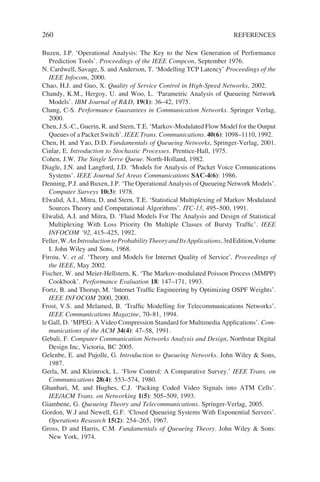
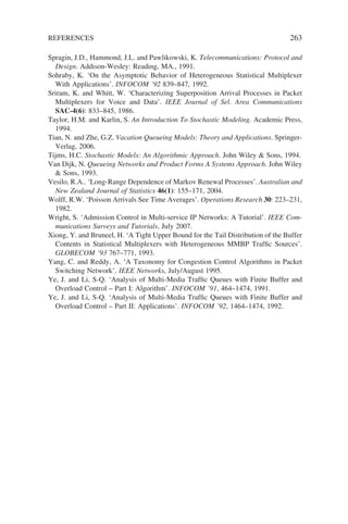
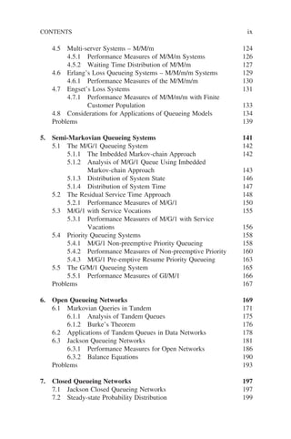
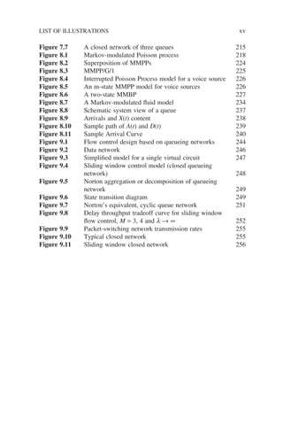
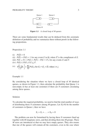
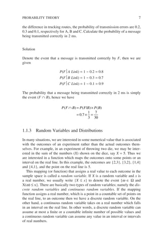
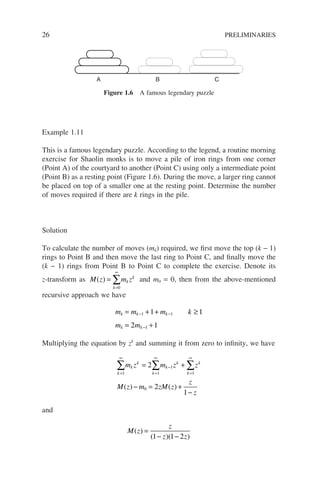
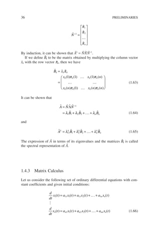
For a discrete random variable, its probability distribution function is a dis-
joint step function, as shown in Figure 1.3. The probability that the random
variable takes on a particular value, say x and x = 0, 1, 2, 3 . . . , is given by
p x P X x P X x P X x
P X x P X x
P X x
( ) [ ] [ ] [ ]
{ [ ]} { [ ]}
[ ]
≡ = = + −
= − ≥ + − − ≥
= ≥
1
1 1 1
−
− ≥ +
P X x
[ ]
1 (1.8)
The above function p(x) is known as the probability mass function (pmf) of a
discrete random variable X and it follows the axiom of probability that
F(x)
1 2
P[X=2]
3 4 x
Figure 1.3 Distribution function of a discrete random variable X](https://image.slidesharecdn.com/qtts-230925120453-047b3b23/85/QTTS-pdf-31-320.jpg)
![x
p x
∑ =
( ) 1 (1.9)
This probability mass function is a more convenient form to manipulate than
the PDF for a discrete random variable.
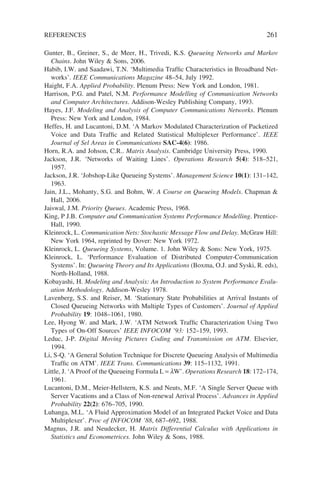
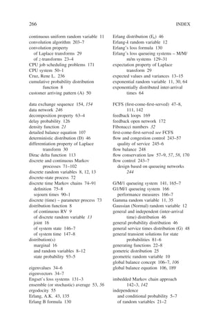
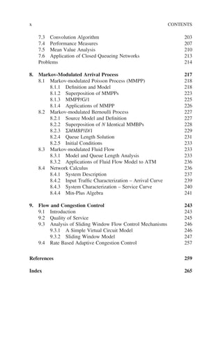
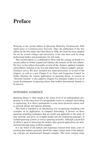
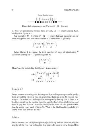
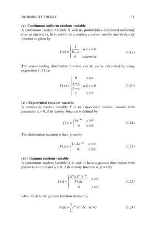
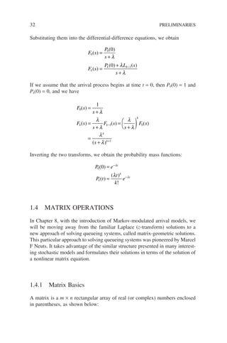
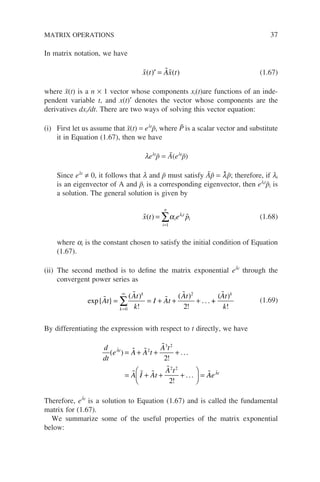
In the case of a continuous random variable, the probability distribution
function is a continuous function, as shown in Figure 1.4, and pmf loses its
meaning as P[X = x] = 0 for all real x.
A new useful function derived from the PDF that completely characterizes
a continuous random variable X is the so-called probability density function
(pdf) defined as
f x
d
dx
F x
X X
( ) ( )
≡ (1.10)
It follows from the axioms of probability and the definition of pdf that
F x f d
X
x
X
( ) ( )
=
−∞
∫ τ τ (1.11)
P a X b f x dx
a
b
X
[ ] ( )
≤ ≤ = ∫ (1.12)
and
−∞
∞
∫ = −∞ ∞ =
f x P X
X( ) [ ] 1 (1.13)
The expressions (1.9) and (1.13) are known as the normalization conditions
for discrete random variables and continuous random variables, respectively.
PROBABILITY THEORY 9
F(x)
1 2 3 4 x
Figure 1.4 Distribution function of a continuous RV](https://image.slidesharecdn.com/qtts-230925120453-047b3b23/85/QTTS-pdf-32-320.jpg)
![10 PRELIMINARIES
We list in this section some important discrete and continuous random vari-
ables which we will encounter frequently in our subsequent studies of queueing
models.
(i) Bernoulli random variable
A Bernoulli trial is a random experiment with only two outcomes, ‘success’
and ‘failure’, with respective probabilities, p and q. A Bernoulli random vari-
able X describes a Bernoulli trial and assumes only two values: 1 (for success)
with probability p and 0 (for failure) with probability q:
P X p P X q p
[ ] [ ]
= = = = = −
1 0 1 (1.14)
(ii) Binomial random variable
If a Bernoulli trial is repeated k times then the random variable X that counts
the number of successes in the k trials is called a binomial random variable
with parameters k and p. The probability mass function of a binomial random
variable is given by
B k n p
n
k
p q k n q p
k n k
( ; )
, , , , . . . ,
=
= = −
−
0 1 2 1 (1.15)
(iii) Geometric random variable
In a sequence of independent Bernoulli trials, the random variable X that counts
the number of trials up to and including the first success is called a geometric
random variable with the following pmf:
P X k p p k
k
[ ] ( )
= = − = ∞
−
1 1 2
1
, ,... (1.16)
(iv) Poisson random variable
A random variable X is said to be Poisson random variable with parameter l
if it has the following mass function:
P X k
k
e k
k
[ ]
!
= = =
−
λ λ
0 1 2
, , , . . . (1.17)
Students should note that in subsequent chapters, the Poisson mass function
is written as
P X k
t
k
e k
k
t
[ ]
( )
!
= =
′
=
− ′
λ λ
0 1 2
, , , . . . (1.18)
Here, the l in expression (1.17) is equal to the l′t in expression (1.18).](https://image.slidesharecdn.com/qtts-230925120453-047b3b23/85/QTTS-pdf-33-320.jpg)
![variable. However, we are also often interested in certain measures which sum-
marize the properties of a random variable succinctly. In fact, often these are
the only parameters that we can observe about a random variable in real-life
problems.
The most important and useful measures of a random variable X are its
expected value1
E[X] and variance Var[X]. The expected value is also known
as the mean value or average value. It gives the average value taken by a
random variable and is defined as
E X kP X k
k
[ ] [ ]
= =
=
∞
∑
0
for discrete variables (1.28)
and E X xf x dx
[ ] ( )
=
∞
∫
0
for continuous variables (1.29)
The variance is given by the following expressions. It measures the disper-
sion of a random variable X about its mean E[X]:
σ2
2
2 2
=
= −
= −
Var X
E X E X
E X E X
[ ]
[( [ ]) ]
[ ] ( [ ])
for discrete variables (1.30)
σ2
0
2
0
2
0 0
2
=
= −
= − +
∞
∞ ∞
∫
∫ ∫
Var X
x E X f x dx
x f x dx E X xf x dx
[ ]
( [ ]) ( )
( ) [ ] ( )
∞
∞
∫
= −
f x dx
E X E X
( )
[ ] ( [ ])
2 2
(1.31)
s refers to the square root of the variance and is given the special name of
standard deviation.
Example 1.4
For a discrete random variable X, show that its expected value is also given by
E X P X k
k
[ ] [ ]
=
=
∞
∑
0
PROBABILITY THEORY 13
for continuous variables
1
For simplicity, we assume here that the random variables are non-negative.](https://image.slidesharecdn.com/qtts-230925120453-047b3b23/85/QTTS-pdf-36-320.jpg)
![14 PRELIMINARIES
Solution
By definition, the expected value of X is given by
E X kP X k k P X k P X k
k k
[ ] [ ] { [ ] [ ]}
= = = ≥ − ≥ +
=
∞
=
∞
∑ ∑
0 0
1 (see (1.8))
= ≥ − ≥ + ≥ − ≥
+ ≥ − ≥ + ≥ −
P X X P X P X
P X P X P X P X
[ ] [ ] [ ] [ ]
[ ] [ ] [ ] [
1 2 2 2 2 3
3 3 3 4 4 4 4 ≥
≥ +
= ≥ =
=
∞
=
∞
∑ ∑
5
1 0
]
[ ] [ ]
. . .
k k
P X k P X k
Example 1.5
Calculate the expected values for the Binomial and Poisson random
variables.
Solution
1. Binomial random variable
E X k
n
k
p p
np
n
k
p P
k
n
k n k
k
n
k
[ ] ( )
( )
=
−
=
−
−
−
=
−
=
−
∑
∑
1
1
1
1
1
1
1 n
n k
j
n
j n j
np
n
j
p p
np
−
=
− −
=
−
−
=
∑
0
1
1
1
( )( )
2. Poisson random variable
E X k
k
e
e
k
e e
k
k
k
k
[ ]
!
( )
( )
( )!
( )
=
=
−
=
=
=
∞
−
−
=
∞ −
−
∑
∑
0
1
1
1
λ
λ
λ
λ
λ
λ
λ
λ λ](https://image.slidesharecdn.com/qtts-230925120453-047b3b23/85/QTTS-pdf-37-320.jpg)
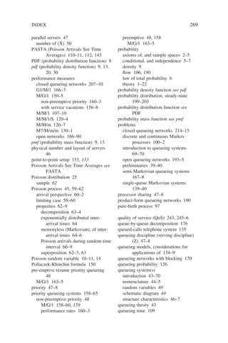
![Table 1.1 summarizes the expected values and variances for those random
variables discussed earlier.
Example 1.6
Find the expected value of a Cauchy random variable X, where the density
function is defined as
f x
x
u x
( )
( )
( )
=
+
1
1 2
π
where u(x) is the unit step function.
Solution
Unfortunately, the expected value of E[X] in this case is
E X
x
x
u x dx
x
x
dx
[ ]
( )
( )
( )
=
+
=
+
= ∞
−∞
∞ ∞
∫ ∫
π π
1 1
2 0 2
Sometimes we get unusual results with expected values, even though the
distribution of the random variable is well behaved.
Another useful measure regarding a random variable is the coefficient of
variation which is the ratio of standard deviation to the mean of that random
variable:
C
E X
x
X
≡
σ
[ ]
PROBABILITY THEORY 15
Table 1.1 Means and variances of some common random
variables
Random variable E[X] Var[X]
Bernoulli p pq
Binomial np npq
Geometric 1/p q/p2
Poisson l l
Continuous uniform (a + b)/2 (b − a)2
/12
Exponential 1/l 1/l2
Gamma a/l a/l2
Erlang-k 1/l 1/kl2
Gaussian m s2
X](https://image.slidesharecdn.com/qtts-230925120453-047b3b23/85/QTTS-pdf-38-320.jpg)
![16 PRELIMINARIES
1.1.5 Joint Random Variables and Their Distributions
In many applications, we need to investigate the joint effect and relationships
between two or more random variables. In this case we have the natural
extension of the distribution function to two random variables X and Y, namely
the joint distribution function. Given two random variables X and Y, their joint
distribution function is defined as
F x y P X x Y y
XY( ) [ ]
, ,
≡ ≤ ≤ (1.32)
where x and y are two real numbers. The individual distribution function FX
and FY, often referred to as the marginal distribution of X and Y, can be
expressed in terms of the joint distribution function as
F x F x P X x Y
F y F y P X Y y
X XY
Y XY
( ) ( [ ]
( ) ( ) [ ]
= ∞ = ≤ ≤ ∞
= ∞ = ≤ ∞ ≤
, ) ,
, , (1.33)
Similar to the one-dimensional case, the joint distribution also enjoys the
following properties:
(i) FXY(−∞, y) = FXY(x, −∞) = 0
(ii) FXY(−∞, −∞) = 0 and FXY(∞, ∞) = 1
(iii) FXY(x1, y) ≤ FXY(x2, y) for x1 ≤ x2
(iv) FXY(x, y1) ≤ FXY(x, y2) for y1 ≤ y2
(v) P[x1 X ≤ x2, y1 Y ≤ y2] = FXY(x2, y2) − FXY(x1, y2)
− FXY(x2, y1) + FXY(x1, y1)
If both X and Y are jointly continuous, we have the associated joint density
function defined as
f x y
d
dxdy
F x y
XY XY
( ) ( )
, ,
≡
2
(1.34)
and the marginal density functions and joint probability distribution can be
computed by integrating over all possible values of the appropriate variables:
f x f x y dy
f y f x y dx
X XY
Y XY
( ) ( )
( ) ( )
=
=
−∞
∞
−∞
∞
∫
∫
,
, (1.35)](https://image.slidesharecdn.com/qtts-230925120453-047b3b23/85/QTTS-pdf-39-320.jpg)
![F x y f u v dudv
XY
x y
XY
( ) ( )
, ,
=
−∞−∞
∫ ∫
If both are jointly discrete then we have the joint probability mass function
defined as
p x y P X x Y y
( ) [ ]
, ,
≡ = = (1.36)
and the corresponding marginal mass functions can be computed as
P X x p x y
P Y y p x y
y
x
[ ] ( )
[ ] ( )
= =
= =
∑
∑
,
, (1.37)
With the definitions of joint distribution and density function in place,
we are now in a position to extend the notion of statistical independence
to two random variables. Basically, two random variables X and Y are said
to be statistically independent if the events {x ∈ E} and {y ∈ F} are inde-
pendent, i.e.:
P[x ∈ E, y ∈ F] = P[x ∈ E]·P[y ∈ F]
From the above expression, it can be deduced that X and Y are statistically
independent if any of the following relationships hold:
• FXY(x, y) = FX(x)·FY(y)
• fXY(x, y) = fX(x)·fY(y) if both are jointly continuous
• P[x = x, Y = y] = P[X = x]·P[Y = y] if both are jointly discrete
We summarize below some of the properties pertaining to the relationships
between two random variables. In the following, X and Y are two independent
random variables defined on the same sample space, c is a constant and g and
h are two arbitrary real functions.
(i) Convolution Property
If Z = X + Y, then
• if X and Y are jointly discrete
P Z k P X i P Y j P X i P Y k i
i j k i
k
[ ] [ ] [ ] [ ] [ ]
= = = = = = = −
+ = =
∑ ∑
0
(1.38)
PROBABILITY THEORY 17](https://image.slidesharecdn.com/qtts-230925120453-047b3b23/85/QTTS-pdf-40-320.jpg)
![18 PRELIMINARIES
• if X and Y are jointly continuous
f z f x f z x dx f z y f y dy
f x f y
Z X Y X Y
X Y
( ) ( ) ( ) ( ) ( )
( ) ( )
= − = −
= ⊗
∞ ∞
∫ ∫
0 0
(1.39)
where ⊗ denotes the convolution operator.
(ii) E[cX] = cE[X]
(iii) E[X + Y] = E[X] + E[Y]
(iv) E[g(X)h(Y)] = E[g(X)]·E[h(Y)] if X and Y are independent
(v) Var[cX] = c2
Var[X]
(vi) Var[X + Y] = Var[X] + Var[Y] if X and Y are independent
(vi) Var[X] = E[X2
] − (E[X])2
Example 1.7: Random sum of random variables
Consider the voice packetization process during a teleconferencing session,
where voice signals are packetized at a teleconferencing station before being
transmitted to the other party over a communication network in packet form.
If the number (N) of voice signals generated during a session is a random vari-
able with mean E(N), and a voice signal can be digitized into X packets,
find the mean and variance of the number of packets generated during a tele-
conferencing session, assuming that these voice signals are identically
distributed.
Solution
Denote the number of packets for each voice signal as Xi and the total number
of packets generated during a session as T, then we have
T = X1 + X2 + . . . + XN
To calculate the expected value, we first condition it on the fact that N = k
and then use the total probability theorem to sum up the probability. That is:
E T E T N k P N k
kE X P N k
E X E N
i
N
i
N
[ ] [ | ] [ ]
[ ] [ ]
[ ] [ ]
= = =
= =
=
=
=
∑
∑
1
1](https://image.slidesharecdn.com/qtts-230925120453-047b3b23/85/QTTS-pdf-41-320.jpg)
![To compute the variance of T, we first compute E[T2
]:
E T N k Var T N k E T N k
kVar X k E X
[ | ] [ | ] ( [ | ])
[ ] ( [ ])
2 2
2 2
= = = + =
= +
and hence we can obtain
E T kVar X k E X P N k
Var X E N E N E X
k
N
[ ] ( [ ] ( [ ]) ) [ ]
[ ] [ ] [ ]( [ ]
2
1
2 2
2
= + =
= +
=
∑
)
)2
Finally:
Var T E T E T
Var X E N E N E X E X E N
[ ] [ ] ( [ ])
[ ] [ ] [ ]( [ ]) ( [ ]) ( [ ])
= −
= + −
2 2
2 2 2 2
2
2
= +
Var X E N E X Var N
[ ] [ ] ( [ ]) [ ]
Example 1.8
Consider two packet arrival streams to a switching node, one from a voice
source and the other from a data source. Let X be the number of time slots until
a voice packet arrives and Y the number of time slots till a data packet arrives.
If X and Y are geometrically distributed with parameters p and q respectively,
find the distribution of the time (in terms of time slots) until a packet arrives
at the node.
Solution
Let Z be the time until a packet arrives at the node, then Z = min(X, Y) and we
have
P Z k P X k P Y k
F k F k F k
Z X Y
[ ] [ ] [ ]
( ) { ( )}{ ( )}
=
− = − −
1 1 1
but
F k p p p
p
p
p
X
j
j
k
k
( ) ( )
( )
( )
( )
= − =
− −
− −
= − −
=
∞
−
∑
1
1
1
1 1
1 1
1 1
PROBABILITY THEORY 19](https://image.slidesharecdn.com/qtts-230925120453-047b3b23/85/QTTS-pdf-42-320.jpg)
![20 PRELIMINARIES
Similarly
FY(k) = 1 − (1 − q)k
Therefore, we obtain
F k p q
p q
Z
k k
k
( ) ( ) ( )
[( )( )]
= − − −
= − − −
1 1 1
1 1 1
Theorem 1.1
Suppose a random variable Y is a function of a finite number of independent
random variables {Xi}, with arbitrary known probability density functions
(pdf). If
Y Xi
=
=
∑
i
n
1
then the pdf of Y is given by the density function:
g y f x f x f x f x
Y X X X Xn n
( ) ( ) ( ) ( ) ( )
= ⊗ ⊗ ⊗
1 1 2 2 3 3 ... (1.40)
The keen observer might note that this result is a general extension of expres-
sion (1.39). Fortunately the convolution of density functions can be easily
handled by transforms (z or Laplace).
Example 1.9
Suppose the propagation delay along a link follows the exponential
distribution:
fX(xi) = exp(−xi) for xi ≥ 0 for i = 1 . . . 10.
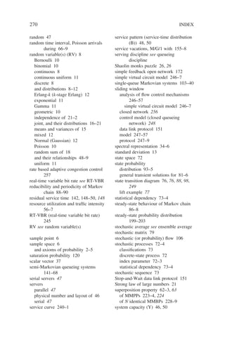
Find the density function g(y) where y = x1+ x2+ . . . x10.
Solution
Consider the effect of the new random variable by using Theorem 1.1 above,
where each exponential random variable are independent and identically
distributed with g(y) =
y e
i
i y
− −
−
1
1
( )!
for y ≥ 0 as shown in Figure 1.5.](https://image.slidesharecdn.com/qtts-230925120453-047b3b23/85/QTTS-pdf-43-320.jpg)
![1.1.6 Independence of Random Variables
Independence is probably the most fertile concept in probability theorems, for
example, it is applied to queueing theory under the guise of the well-known
Kleinrock independence assumption.
Theorem 1.2
[Strong law of large numbers]
For n independent and identically distributed random variables {Xn, n ≥ 1}:
Y X X X n E X n
n n
= + → → ∞
{ } [ ]
1 2 1
... / as (1.41)
That is, for large n, the arithmetic mean of Yn of n independent and identically
distributed random variables with the same distribution is close to the expected
value of these random variables.
Theorem 1.3
[Central Limit theorem]
Given Yn as defined above:
PROBABILITY THEORY 21
0 2 4 6 8 10 12 14 16 18 20
0
0.1
0.2
0.3
0.4
0.5
0.6
0.7
0.8
0.9
1
y
g(y)
Figure 1.5 The density function g(y) for I = 1 . . . 10](https://image.slidesharecdn.com/qtts-230925120453-047b3b23/85/QTTS-pdf-44-320.jpg)
![22 PRELIMINARIES
{ [ ]} ( )
Y E X n N n
n − ≈
1
2
0 1
, for
σ (1.42)
where N(0,s2
) denotes the random variable with mean zero and variance s2
of each Xn.
The theorem says that the difference between the arithmetic mean of Yn and
the expected value E[X1] is a Gaussian distributed random variable divided by
n for large n.
1.2 z-TRANSFORMS – GENERATING FUNCTIONS
If we have a sequence of numbers {f0, f1, f2, . . . fk . . .}, possibly infinitely long,
it is often desirable to compress it into a single function – a closed-form expres-
sion that would facilitate arithmetic manipulations and mathematical proofing
operations. This process of converting a sequence of numbers into a single
function is called the z-transformation, and the resultant function is called the
z-transform of the original sequence of numbers. The z-transform is commonly
known as the generating function in probability theory.
The z-transform of a sequence is defined as
F z f z
k
k
k
( ) ≡
=
∞
∑
0
(1.43)
where zk
can be considered as a ‘tag’ on each term in the sequence and hence
its position in that sequence is uniquely identified should the sequence need to
be recovered. The z-transform F(z) of a sequence exists so long as the sequence
grows slower than ak
, i.e.:
lim
k
k
k
k
a
→∞
= 0
for some a 0 and it is unique for that sequence of numbers.
z-transform is very useful in solving difference equations (or so-called recur-
sive equations) that contain constant coefficients. A difference equation is an
equation in which a term (say kth) of a function f(•) is expressed in terms of
other terms of that function. For example:
fk−1 + fk+1 = 2fk
This kind of difference equation occurs frequently in the treatment of queueing
systems. In this book, we use ⇔ to indicate a transform pair, for example,
fk ⇔ F(z).](https://image.slidesharecdn.com/qtts-230925120453-047b3b23/85/QTTS-pdf-45-320.jpg)
![24 PRELIMINARIES
(c) Final values and expectation
(i) F z z
( ) = =
1 1 (1.46)
(ii) E X
d
dz
F z z
[ ] ( )
= =1
(1.47)
(iii) E X
d
dz
F z
d
dz
F z
z z
[ ] ( ) ( )
2
2
2 1 1
= +
= =
(1.48)
Table 1.2 summarizes some of the z-transform pairs that are useful in our sub-
sequent treatments of queueing theory.
Example 1.10
Let us find the z-transforms for Binomial, Geometric and Poisson distributions
and then calculate the expected values, second moments and variances for these
distributions.
(i) Binomial distribution:
B z
n
k
p p z
p pz
d
dz
B z np p p
X
k
n
k n k k
n
X
( ) ( )
( )
( ) (
=
−
= − +
= − +
=
−
∑
0
1
1
1 z
z n
) −1
therefore
E X
d
dz
B z np
X z
[ ] ( )
= =
=1
Table 1.2 Some z-transform pairs
Sequence z-transform
uk = 1k = 0, 1, 2 . . . 1/(1 − z)
uk−a za
/(1 − z)
Aak
A/(1 − az)
kak
az/(1 − az)2
(k + 1)ak
1/(1 − az)2
a/k! aez](https://image.slidesharecdn.com/qtts-230925120453-047b3b23/85/QTTS-pdf-47-320.jpg)
![and
d
dz
B z np n p p pz
E X n n p np
E X E
X
n
2
2
2
2 2
2 2 2
1 1
1
( ) ( ) ( )
[ ] ( )
[ ]
= − − +
= − +
= −
−
σ [
[ ]
( )
X
np p
= −
1
(ii) Geometric distribution:
G z p p z
pz
p z
E X
p
p z
pz p
k
k k
( ) ( )
( )
[ ]
( )
( )
( (
= − =
− −
=
− −
+
−
−
=
∞
−
∑
1
1
1
1 1
1 1
1
1 1
1
1
2
1 1
1 1
2
1
2
2
1
2
2
2
−
=
= −
= −
=
=
p z p
d
dz
G z
p p
p p
z
z
) )
( )
σ
(iii) Poisson distribution:
G z
t
k
e z e e e
E X
d
dz
G z
k
k
t k t tz t z
z
( )
( )
!
[ ] ( )
( )
= = =
=
=
∞
− − + − −
=
∑
0
1
1
λ λ λ λ λ
=
= =
=
= − =
− −
=
λ λ
λ
σ λ
λ
te t
d
dz
G z t
E X E X t
t z
z
( )
( ) ( )
[ ] [ ]
1
2
2
1
2
2 2 2
Table 1.3 summarizes the z-transform expressions for those probability mass
functions discussed in Section 1.2.3.
z-TRANSFORMS – GENERATING FUNCTIONS 25
Table 1.3 z-transforms for some of the discrete random
variables
Random variable z-transform
Bernoulli G(z) = q + pz
Binomial G(z) = (q + pz)n
Geometric G(z) = pz/(1 − qz)
Poisson G(z) = e−lt(1−z)](https://image.slidesharecdn.com/qtts-230925120453-047b3b23/85/QTTS-pdf-48-320.jpg)
![To find the inverse of this expression, we do a partial fraction expansion:
M z
z z
z z z
( ) ( ) ( ) ( )
=
−
+
−
−
= − + − + − +
1
1 2
1
1
2 1 2 1 2 1
2 2 3 3
. . .
Therefore, we have mk = 2k
− 1
Example 1.12
Another well-known puzzle is the Fibonacci numbers {1, 1, 2, 3, 5, 8, 13, 21,
. . .}, which occur frequently in studies of population grow. This sequence of
numbers is defined by the following recursive equation, with the initial two
numbers as f0 = f1 = 1:
fk = fk−1 + fk−2 k ≥ 2
Find an explicit expression for fk.
Solution
First multiply the above equations by zk
and sum it to infinity, so we have
k
k
k
k
k
k
k
k
k
f z f z f z
F z f z f z F z f z
=
∞
=
∞
−
=
∞
−
∑ ∑ ∑
= +
− − = − +
2 2
1
2
2
1 0 0
2
( ) ( ( ) ) F
F z
F z
z z
( )
( ) =
−
+ −
1
1
2
Again, by doing a partial fraction expression, we have
F z
z z z z z z
z
z
z z
( )
[ ( / )] [ ( / )]
=
−
−
−
= + +
−
1
5 1
1
5 1
1
5
1
1
5
1
1 1 2 2
1 1 2
... +
+ +
z
z2
...
where
z z
1 2
1 5
2
1 5
2
=
− +
=
− −
and
z-TRANSFORMS – GENERATING FUNCTIONS 27](https://image.slidesharecdn.com/qtts-230925120453-047b3b23/85/QTTS-pdf-50-320.jpg)
![28 PRELIMINARIES
Therefore, picking up the k term, we have
fk
k k
=
+
−
−
+ +
1
5
1 5
2
1 5
2
1 1
1.3 LAPLACE TRANSFORMS
Similar to z-transform, a continuous function f(t) can be transformed into
a new complex function to facilitate arithmetic manipulations. This trans-
formation operation is called the Laplace transformation, named after the
great French mathematician Pierre Simon Marquis De Laplace, and is
defined as
F s L f t f t e dt
st
( ) [ ( )] ( )
= =
−∞
∞
−
∫ (1.49)
where s is a complex variable with real part s and imaginary part jw; i.e.
s = s + jw and j = −1. In the context of probability theory, all the density
functions are defined only for the real-time axis, hence the ‘two-sided’ Laplace
transform can be written as
F s L f t f t e dt
st
( ) [ ( )] ( )
= =
−
∞
−
∫
0
(1.50)
with the lower limit of the integration written as 0−
to include any discontinuity
at t = 0. This Laplace transform will exist so long as f(t) grows no faster than
an exponential, i.e.:
f(t) ≤ Meat
for all t ≥ 0 and some positive constants M and a. The original function f(t) is
called the inverse transform or inverse of F(s), and is written as
f(t) = L−1
[F(s)]
The Laplace transformation is particularly useful in solving differential equa-
tions and corresponding initial value problems. In the context of queueing
theory, it provides us with an easy way of finding performance measures of a
queueing system in terms of Laplace transforms. However, students should
note that it is at times extremely difficult, if not impossible, to invert these
Laplace transform expressions.](https://image.slidesharecdn.com/qtts-230925120453-047b3b23/85/QTTS-pdf-51-320.jpg)
![1.3.1 Properties of the Laplace Transform
The Laplace transform enjoys many of the same properties as the z-
transform as applied to probability theory. If X and Y are two independent
continuous random variables with density functions fX(x) and fY(y),
respectively and their corresponding Laplace transforms exist, then their
properties are:
(i) Uniqueness property
f f F s F s
X Y X Y
( ) ( ) ( ) ( )
τ τ
= =
implies (1.51)
(ii) Linearity property
af x bf y aF s bF s
X Y X Y
( ) ( ) ( ) ( )
+ ⇒ + (1.52)
(iii) Convolution property
If Z = X + Y, then
F s L f z L f x y
F s F s
Z z X Y
X Y
( ) [ ( )] [ ( )]
( ) ( )
= = +
= ⋅
+
(1.53)
(iv) Expectation property
E X
d
ds
F s E X
d
ds
F s
X s X s
[ ] ( ) [ ] ( )
= − =
= =
0
2
2
2 0
and (1.54)
E X
d
ds
F s
n n
n
n X s
[ ] ( ) ( )
= − =
1 0
(1.55)
(v) Differentiation property
L f x sF s f
X X X
[ ( )] ( ) ( )
′ = − 0 (1.56)
L f x s F s sf f
X X X X
[ ( )] ( ) ( ) ( )
′′ = − − ′
2
0 0 (1.57)
Table 1.4 shows some of the Laplace transform pairs which are useful in our
subsequent discussions on queueing theory.
LAPLACE TRANSFORMS 29](https://image.slidesharecdn.com/qtts-230925120453-047b3b23/85/QTTS-pdf-52-320.jpg)
![30 PRELIMINARIES
Example 1.13
Derive the Laplace transforms for the exponential and k-stage Erlang probabil-
ity density functions, and then calculate their means and variances.
(i) exponential distribution
F s e e dx
s
e
s
ss x s x
( ) ( )
= = −
+
=
+
∞
− − − +
∞
∫
0 0
λ
λ
λ
λ
λ
λ λ
F s e e dx
s
e
s
E X
d
ds
F s
sx x s x
( )
[ ] (
( )
= = −
+
=
+
= −
∞
− − − +
∞
∫
0 0
λ
λ
λ
λ
λ
λ λ
)
)
[ ] ( )
[ ] [ ]
[ ]
s
s
E X
d
ds
F S
E X E X
C
E X
=
=
=
= =
= − =
= =
0
2
2
2
0
2
2 2 2
2
1
2
1
1
λ
λ
σ
λ
σ
(ii) k-stage Erlang distribution
F s e
x
k
e dx
k
x e dx
ss
k k
x
k
k s x
( )
( )! ( )!
( )
=
−
=
−
=
∞
−
−
−
∞
− − +
∫ ∫
0
1
0
1
1 1
λ λ
λ
λ λ
k
k
k
k s x
s k
s x e d s x
( ) ( )!
{( ) } ( )
( )
+ −
+ +
∞
− − +
∫
λ
λ λ
λ
1 0
1
Table 1.4 Some Laplace transform pairs
Function Laplace transform
d(t) unit impulse 1
d(t − a) e−as
1 unit step 1/s
t 1/s2
tn−1
/(n − 1)! 1/sn
Aeat
A/(s − a)
teat
1/(s − a)2
tn−1
eat
/(n − 1)! 1/(s − a)n
n = 1,2, . . .](https://image.slidesharecdn.com/qtts-230925120453-047b3b23/85/QTTS-pdf-53-320.jpg)
![The last integration term is recognized as the gamma function and is equal to
(k − 1)! Hence we have
F s
s
k
( ) =
+
)
λ
λ
Table 1.5 gives the Laplace transforms for those continuous random variables
discussed in Section 1.1.3.
Example 1.14
Consider a counting process whose behavior is governed by the following two
differential-difference equations:
d
dt
P t P t P t k
d
dt
P t P t
k k k
( ) ( ) ( )
( ) ( )
= − +
= −
−
λ λ
λ
1
0 0
0
Where Pk(t) is the probability of having k arrivals within a time interval (0, t)
and l is a constant, show that Pk(t) is Poisson distributed.
Let us define the Laplace transform of Pk(t) and P0(t) as
F s e P t dt
F s e P t dt
k
st
k
st
( ) ( )
( ) ( )
=
=
∞
−
∞
−
∫
∫
0
0
0
0
From the properties of Laplace Transform, we know
L P t sF s P
L P t sF s P
k k k
[ ( )] ( ) ( )
[ ( )] ( ) ( )
′ = −
′ = −
0
0
0 0 0
LAPLACE TRANSFORMS 31
Table 1.5 Laplace transforms for some probability
functions
Random variable Laplace transform
Uniform a x b F(s) = e−s(a+b)
/s(b − a)
Exponent F(s) = l/s + l
Gamma F(s) = la
/(s + l)a
Erlang-k F(s) = lk
/(s + l)k](https://image.slidesharecdn.com/qtts-230925120453-047b3b23/85/QTTS-pdf-54-320.jpg)
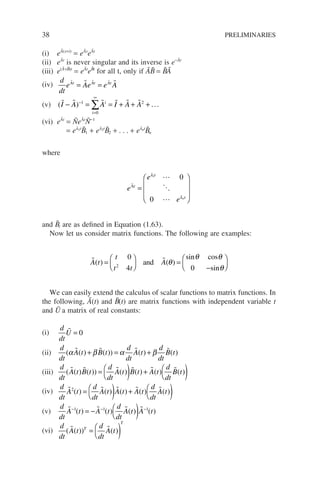
![A has n eigenvalues l1, l2, . . . , ln with the corresponding eigenvectors x̃1,
x̃2, . . . , x̃n. The polynomial is known as the characteristic polynomial of A and
the set of eigenvalues is called the spectrum of Ã.
Similarly, the row (or left) eigenvectors are the solutions of the following
vector equation:
π λπ
A = (1.59)
and everything that is said about column eigenvectors is also true for row
eigenvectors.
Here, we summarize some of the properties of eigenvalues and
eigenvectors:
(i) The sum of the eigenvalues of à is equal to the sum of the diagonal entries
of Ã. The sum of the diagonal entries of à is called the trace of Ã.
tr A
i
i
( )
= ∑λ (1.60)
(ii) If A has eigenvalues l1, l2, . . . , ln, then lk
1, lk
2, . . . , lk
n are eigenvectors
of Ãk
, and we have
tr A k
k
i
i
k
( )
= =
∑λ 1 2
, , . . . (1.61)
(iii) If à is a non-singular matrix with eigenvalues l1, l2, . . . ,ln, then
l1
−1
, l2
−1
), . . . , ln
−1
are eigenvectors of Ã−1
. Moreover, any eigenvector
of à is an eigenvector of Ã−1
.
(iv) Ã and ÃT
do not necessarily have the same eigenvectors. However, if
ÃT
x̃ = lx̃ then x̃T
à = lx̃T
, and the row vector x̃T
is called a left eigenvector
of Ã.
It should be pointed out that eigenvalues are in general relatively difficult to
compute, except for certain special cases.
If the eigenvalues l1, l2, . . . , ln of a matrix à are all distinct, then the cor-
responding eigenvectors x̃1, x̃2, ..., x̃n are linearly independent, and we can
express à as
A N N
= −
Λ 1
(1.62)
where Λ̃= diag(l1, l2, . . . , ln), Ñ = [x̃1, x̃2, . . . , x̃n] whose ith column is x̃i, Ñ−1
is the inverse of Ñ, and is given by
MATRIX OPERATIONS 35](https://image.slidesharecdn.com/qtts-230925120453-047b3b23/85/QTTS-pdf-58-320.jpg)
![Problems
1. A pair of fair dice is rolled 10 times. What will be the probability that
‘seven’ will show at least once.
2. During Christmas, you are provided with two boxes A and B contain-
ing light bulbs from different vendors. Box A contains 1000 red bulbs
of which 10% are defective while Box B contains 2000 blue bulbs
of which 5% are defective.
(a) If I choose two bulbs from a randomly selected box, what is the
probability that both bulbs are defective?
(b) If I choose two bulbs from a randomly selected box and find that
both bulbs are defective, what is the probability that both came
from Box A?
3. A coin is tossed an infinite number of times. Show that the probabil-
ity that k heads are observed at the nth tossing but not earlier equals
n
k
n
−
−
− −
1
1
1
p p)
k k
( , where p = P{H}.
4. A coin with P{H} = p and P{T} = q = 1 − p is tossed n times.
Show that the probability of getting an even number of heads is
0.5[1 + (q − p)n
].
5. Let A, B and C be the events that switches a, b and c are closed,
respectively. Each switch may fail to close with probability q. Assume
that the switches are independent and find the probability that a
closed path exists between the terminals in the circuit shown for
q = 0.5.
6. The binary digits that are sent from a detector source generate bits
1 and 0 randomly with probabilities 0.6 and 0.4, respectively.
(a) What is the probability that two 1 s and three 0 s will occur in
a 5-digit sequence.
(b) What is the probability that at least three 1 s will occur in a 5-
digit sequence.
MATRIX OPERATIONS 39
a
b
c
Figure 1.7 Switches for Problem 6](https://image.slidesharecdn.com/qtts-230925120453-047b3b23/85/QTTS-pdf-62-320.jpg)

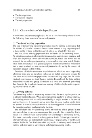
![Looking at the structure of a queueing system, we can easily arrive at the
following expressions:
N t N t N t N N N
q s q s
( ) ( ) ( )
= + = +
and (2.1)
T W x T W x
k k k
= + = +
and (2.2)
If the queueing system in question is ergodic (a concept that we shall explain
later in Section 2.4.2) and has reached the steady state, then the following
expressions hold:
N N t E N t
t t
= =
→∞ →∞
lim lim
( ) [ ( )] (2.3)
N N t E N t
q
t
q
t
q
= =
→∞ →
lim lim
( ) [ ( )] (2.4)
N N t E N t
s
t
s
t
s
= =
→∞ →∞
lim lim
( ) [ ( )] (2.5)
T T E T
k
k
k
k
= = [ ]
→∞ →∞
lim lim (2.6)
W W E W
k
k
k
k
= =
→∞ →∞
lim lim [ ] (2.7)
x x E x
k
k
k
k
= =
→∞ →∞
lim lim [ ] (2.8)
P P t
k
t
k
=
→∞
lim ( ) (2.9)
Table 2.1 Random variables of a queueing system
Notation Description
N(t) The number of customers in the system at time t
Nq(t) The number of customers in the waiting queue at time t
Ns(t) The number of customers in the service facility at time t
N The average number of customers in the system
Nq The average number of customers in the waiting queue
Ns The average number of customers in the service facility
Tk The time spent in the system by kth customer
Wk The time spent in the waiting queue by kth customer
xk The service time of kth customer
T The average time spent in the system by a customer
W The average time spent in the waiting queue by a customer
x̄ The average service time
Pk(t) The probability of having k customers in the system at time t
Pk The stationary probability of having k customers in the system
RANDOM VARIABLES AND THEIR RELATIONSHIPS 49](https://image.slidesharecdn.com/qtts-230925120453-047b3b23/85/QTTS-pdf-72-320.jpg)
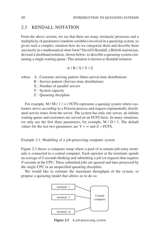
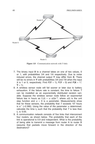
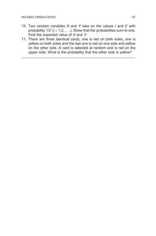
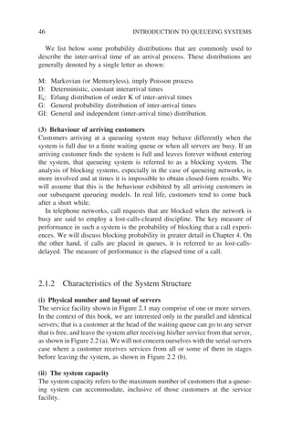
![52 INTRODUCTION TO QUEUEING SYSTEMS
2.4 LITTLE’S THEOREM
Before we examine the stochastic behaviour of a queueing system, let us first
establish a very simple and yet powerful result that governs its steady-state
performance measures – Little’s theorem, law or result are the various names.
This result existed as an empirical rule for many years and was first proved in
a formal way by J D C Little in 1961 (Little 1961).
This theorem relates the average number of customers (N) in a steady-state
queueing system to the product of the average arrival rate (l) of customers
entering the system and the average time (T) a customer spent in that system,
as follows:
N T
= λ (2.11)
This result was derived under very general conditions. The beauty of it lies
in the fact that it does not assume any specific distribution for the arrival as
well as the service process, nor it assumes any queueing discipline or depends
upon the number of parallel servers in the system. With proper interpretation
of N, l and T, it can be applied to all types of queueing systems, including
priority queueing and multi-server systems.
Here, we offer a simple proof of the theorem for the case when customers
are served in the order of their arrivals. In fact, the theorem holds for any
queueing disciplines as long as the servers are kept busy when the system is
not empty.
Let us count the number of customers entering and leaving the system as
functions of time in the interval (0, t) and define the two functions:
A(t): Number of arrivals in the time interval (0, t)
D(t): Number of departures in the time interval (0, t)
Assuming we begin with an empty system at time 0, then N(t) = A(t) − D(t)
represents the total number of customers in the system at time t. A general
sample pattern of these two functions is depicted in Figure 2.6, where tk is the
instant of arrival and Tk the corresponding time spent in the system by the kth
customer.
It is clear from Figure 2.6 that the area between the two curves A(t) and D(t)
is given by
N d A D d
T t t
t
t
k k
k D t
A t
k
D
( ) [ ( ) ( )]
( )
( )
( )
(
τ τ τ τ τ
= −
= × + − ×
∫
∫
∑
= +
=
0
0
1
1
1 1
t
t)
∑](https://image.slidesharecdn.com/qtts-230925120453-047b3b23/85/QTTS-pdf-75-320.jpg)
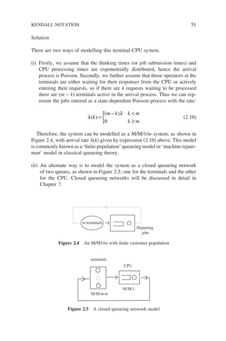
![number of packets in the system (Nsub) is the sum of packets at both the switch
and the transmission line B:
N N N T T
T T T
sub sw B sw B B
sub sw B
= + = +
= +
λ λ
(2.17)
where Tsw is the time spent at the central switch
TB is the time spent by a packet to be transmitted over Line B
Nsw is the number of packets at the switch
NB is the number of packets at Line B
lB is the arrival rate of packets to Line B.
We can also apply Little’s result to the system as a whole (Box 2). Then T and
N are the corresponding quantities of that system:
N T
= λ (2.18)
2.4.2 Ergodicity
Basically, ‘Ergodicity’ is a concept related to the limiting values and stationary
distribution of a long sample path of a stochastic process. There are two ways
of calculating the average value of a stochastic process over a certain time
interval. In experiments, the average value of a stochastic process X(t) is often
obtained by observing the process for a sufficiently long period of time (0 ,T)
and then taking the average as
X
T
X t dt
T
= ∫
1
0
( )
The average so obtained is called the time average. However, a stochastic
process may take different realizations during that time interval, and the par-
ticular path that we observed is only a single realization of that process. In
probability theory, the expected value of a process at time T refers to the
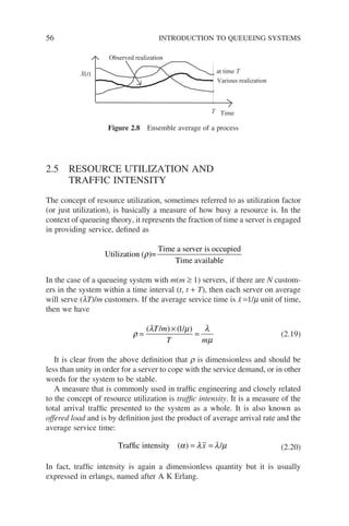
average of the various realizations at time T, as shown in Figure 2.8, and is
given by
E X T kP X T k
k
[ ( )] [ ( ) ]
= =
=
∞
∑
0
This expected value is also known as the ensemble average. For a stochastic
process, if the time average is equal to the ensemble average as T → ∞, we
say that the process is ergodic.
LITTLE’S THEOREM 55](https://image.slidesharecdn.com/qtts-230925120453-047b3b23/85/QTTS-pdf-78-320.jpg)
![Hence, we have
l1 = 2ga + gb
l2 = 2(ga + gb)
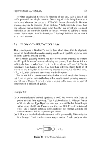
2.7 POISSON PROCESS
Poisson process is central to physical process modelling and plays a pivotal
role in classical queuing theory. In most elementary queueing systems, the
inter-arrival times and service times are assumed to be exponentially distrib-
uted or, equivalently, that the arrival and service processes are Poisson, as we
shall see below. The reason for its ubiquitous use lies in the fact that it pos-
sesses a number of marvellous probabilistic properties that give rise to many
elegant queueing results. Secondly, it also closely resembles the behaviour of
numerous physical phenomenon and is considered to be a good model for an
arriving process that involves a large number of similar and independent
users.
Owing to the important role of Poisson process in our subsequent modelling
of arrival processes to a queueing system, we will take a closer look at it and
examine here some of its marvellous properties.
Put simply, a Poisson process is a counting process for the number of ran-
domly occurring point events observed in a given time interval (0, t). It can
also be deemed as the limiting case of placing at random k points in the time
interval of (0, t). If the random variable X(t) that counts the number of point
events in that time interval is distributed according to the well-known Poisson
distribution given below, then that process is a Poisson process:
P X t k
t
k
e
k
t
[ ( ) ]
( )
!
= = −
λ λ
(2.21)
Here, l is the rate of occurrence of these point events and lt is the mean of a
Poisson random variable and physically it represents the average number of
occurrences of the event in a time-interval t. Poisson distribution is named after
the French mathematician, Simeon Denis Poisson.
2.7.1 The Poisson Process – A Limiting Case
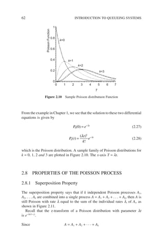
The Poisson process can be considered as a limiting case of the Binomial dis-
tribution of a Bernoulli trial. Assuming that the time interval (0, t) is divided
into time slots and each time slot contains only one point, if we place points
POISSON PROCESS 59](https://image.slidesharecdn.com/qtts-230925120453-047b3b23/85/QTTS-pdf-82-320.jpg)
![60 INTRODUCTION TO QUEUEING SYSTEMS
at random in that interval and consider a point in a time slot as a ‘success’,
then the number of k ‘successes’ in n time slots is given by the Binomial
distribution:
P k n
n
k
p p
k n k
[ ( )
successes in time-slots] =
− −
1
Now let us increase the number of time slots (n) and at the same time
decrease the probability (p) of ‘success’ in such a way that the average number
of ‘successes’ in a time interval t remains constant at np = lt, then we have
the Poisson distribution:
P k t
n
k
t
n
t
n
n
k n k
[ )]
(
arrivals in (0,
lim
=
−
=
→∞
−
λ λ
1
λ
λ λ
t
k
n n n k
n
t
n
k
n k n
n
)
!
( ) ( )
lim
. . .
lim
→∞ →∞
− − +
−
1 1
1
= −
=
→∞
−
−
( )
!
( )
!
λ λ
λ
λ
λ
t
k
t
n
t
k
k
n
n
t
t
k
lim 1
e
e t
−λ
(2.22)
In the above expression, we made use of the identity:
e
t
n
n
n t
= −
→∞
−
lim 1
λ
λ
So we see that the process converges to a Poisson process. Therefore, Poisson
process can be deemed as the superposition of a large number of Bernoulli
arrival processes.
2.7.2 The Poisson Process – An Arrival Perspective
Poisson process has several interpretations and acquires different perspectives
depending on which angle we look at it. It can also be viewed as a counting
process {A(t), t ≥ 0} which counts the number of arrivals up to time t where
A(0) = 0. If this counting process satisfies the following assumptions then it is
a Poisson process.](https://image.slidesharecdn.com/qtts-230925120453-047b3b23/85/QTTS-pdf-83-320.jpg)
![(i) The distribution of the number of arrivals in a time interval depends only
on the length of that interval. That is
P A t t o t
P A t t o t
P A t o t
[ ( ) ] ( )
[ ( ) ] ( )
( ) ( )
∆ ∆ ∆
∆ ∆ ∆
∆ ∆
= = − +
= = +
≥
[ ] =
0 1
1
2
λ
λ
where o(∆t) is a function such that lim
∆
∆
∆
t
o t
t
→
=
0
0
( )
.
This property is known as independent increments.
(ii) The number of arrivals in non-overlapping intervals is statistically inde-
pendent. This property is known as stationary increments.
The result can be shown by examining the change in probability over a time
interval (t, t + ∆t). If we define Pk(t) to be the probability of having k arrivals
in a time interval t and examine the change in probability in that interval,
then
P t t P k arrivals in t t
P k i in t i in t
k
i
k
( ) [ ( )]
[( ) ( ) ]
+ = +
= − 0
=
∑
∆ ∆
∆
0
0
,
,
(2.23)
Using the assumptions (i) and (ii) given earlier:
P t t P k i arrivals in t P i in t
P t t
k
i
k
k
( ) [( ) ( )] [ ]
( )[
+ = − ×
= −
=
∑
∆ ∆
∆
0
0
1
,
λ +
+ + +
−
0 0
1
( )] ( )[ ( )]
∆ ∆ ∆
t P t t t
k λ
(2.24)
Rearranging the terms, we have
Pk (t + ∆t) − Pk(t) = −l∆tPk(t) + l∆tPk−1(t) + O(∆t)
Dividing both equations by ∆t and letting ∆t → 0, we arrive at
dP t
dt
P t P t k
k
k k
( )
( ) ( )
= − +
−
λ λ 1 0 (2.25)
Using the same arguments, we can derive the initial condition:
dP t
dt
P t
0
0
( )
( )
= −λ (2.26)
POISSON PROCESS 61](https://image.slidesharecdn.com/qtts-230925120453-047b3b23/85/QTTS-pdf-84-320.jpg)
![Taking expectations of both sides, we have
E z E Z
E z E z E z
A A A A
A A A
K
k
[ ] = [ ]
= [ ] [ ] [ ]
+ + +
1 2
1 2
...
. . . . (indenpendence
e assumption)
=
=
− − − −
− + + +
e e
e
t z t z
t
k
k
λ λ
λ λ λ
1
1 2
1 1
( ) ( )
( ... ) (
. . . .
1
1−z)
(2.29)
The right-hand side of the final expression is the z-transform of a Poisson
distribution with rate (l1 + l2 + . . . + lk), hence the resultant process is
Poisson.
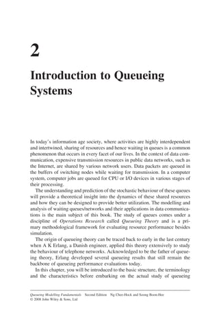
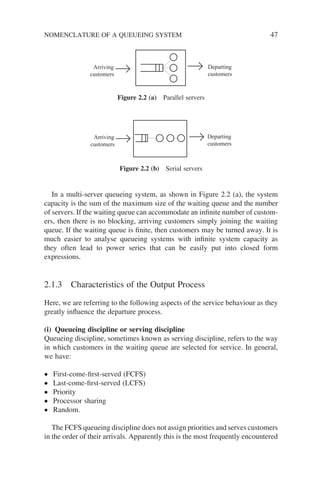
2.8.2 Decomposition Property
The decomposition property is just the reverse of the previous property, as
shown in Figure 2.12, where a Poisson process A is split into k processes using
probability pi (i = 1, . . . , k).
Let us derive the probability mass function of a typical process Ai. On condi-
tion that there are N arrivals during the time interval (0, t) from process A, the
probability of having k arrivals at process Ai is given by
Poisson A1
Poisson Ak
Poisson A
Figure 2.11 Superposition property
Poisson A1
Poisson Ak
Poisson A
P1
Pk
Figure 2.12 Decomposition property
PROPERTIES OF THE POISSON PROCESS 63](https://image.slidesharecdn.com/qtts-230925120453-047b3b23/85/QTTS-pdf-86-320.jpg)
![64 INTRODUCTION TO QUEUEING SYSTEMS
P A t k A t N N k
N
k
P p
i i
k
i
N k
[ ( ) | ( ) ] ( )
= = ≥ =
− −
1 (2.30)
The unconditional probability is then calculated using the total probability
theorem:
P A t k
N
N k k
p p
t
N
e
e
k
p
i
N k
k
i
N k
N
t
t
i
[ ( ) ]
!
( )! !
( )
( )
!
!
= =
−
−
=
=
∞
− −
−
∑ 1 1
λ λ
λ
1
1
1
1
1
−
−
−
=
−
−
=
∞
−
∑
p
p t
N k
e
k
p
p
i
k
N k
i
N
t
i
i
k
[( ) ]
( )!
!
[(
λ
λ
p
p t
p t
j
p t
k
e
i
k
j
i
j
i
k
p t
i
) ]
[( ) ]
!
( )
!
λ
λ
λ λ
=
∞
−
∑
−
=
0
1
(2.31)
That is, a Poisson process with rate pil.
2.8.3 Exponentially Distributed Inter-arrival Times
The exponential distribution and the Poisson process are closely related and in
fact they mirror each other in the following sense. If the inter-arrival times in
a point process are exponentially distributed, then the number of arrival points
in a time interval is given by the Poisson distribution and the process is a
Poisson arrival process. Conversely, if the number of arrival points in any
interval is a Poisson random variable, the inter-arrival times are exponential
distributed and the arrival process is Poisson.
Let t be the inter-arrival time, then
P[t ≤ t] = 1 − P[t t].
But P[t t] is just the probability that no arrival occurs in (0, t); i.e. P0(t).
Therefore we obtain
P t e t
[ ] (
τ λ
≤ = − −
1 exponential distribution) (2.32)
2.8.4 Memoryless (Markovian) Property of Inter-arrival Times
The memoryless property of a Poisson process means that if we observe the
process at a certain point in time, the distribution of the time until next arrival
is not affected by the fact that some time interval has passed since the last](https://image.slidesharecdn.com/qtts-230925120453-047b3b23/85/QTTS-pdf-87-320.jpg)
![arrival. In other words, the process starts afresh at the time of observation and
has no memory of the past. Before we deal with the formal definition, let us
look at an example to illustrate this concept.
Example 2.4
Consider the situation where trains arrive at a station according to a Poisson
process with a mean inter-arrival time of 10 minutes. If a passenger arrives at
the station and is told by someone that the last train arrived 9 minutes ago, so
on the average, how long does this passenger need to wait for the next train?
Solution
Intuitively, we may think that 1 minute is the answer, but the correct answer
is 10 minutes. The reason being that Poisson process, and hence the exponential
inter-arrival time distribution, is memoryless. What have happened before were
sure events but they do not have any influence on future events.
This apparent ‘paradox’ lies in the renewal theory and can be explained
qualitatively as such. Though the average inter-arrival time is 10 minutes, if
we look at two intervals of inter-train arrival instants, as shown in Figure 2.13,
a passenger is more likely to arrive within a longer interval T2 rather than a
short interval of T1. The average length of the interval in which a customer is
likely to arrive is twice the length of the average inter-arrival time. We will
re-visit this problem quantitatively in Chapter 5.
Mathematically, the ‘memoryless’ property states that the distribution of
remaining time until the next arrival, given that t0 units of time have elapsed
since the last arrival, is identically equal to the unconditional distribution of
inter-arrival times (Figure 2.14).
Assume that we start observing the process immediately after an arrival at
time 0. From Equation (2.21) we know that the probability of no arrivals in (0,
t0) is given by
P[no arrival in (0, t0)] = e−lt0
time
T1 T2
train arrival instant
Figure 2.13 Sample train arrival instants
PROPERTIES OF THE POISSON PROCESS 65](https://image.slidesharecdn.com/qtts-230925120453-047b3b23/85/QTTS-pdf-88-320.jpg)
![66 INTRODUCTION TO QUEUEING SYSTEMS
Let us now find the conditional probability that the first arrival occurs in
[t0, t0 + t], given that t0 has elapsed; that is
P arrival in t t t no arrival in t
e
e
t
t t
t
t
[ ( )| ( )]
0 0 0
0 0
0
0
, ,
+ = =
+
−
−
∫ λ λ
λ
1
1− −
e t
λ
But the probability of an arrival in (0, t) is also
0
1
t
t t
e dt e
∫ − −
= −
λ λ λ
Therefore, we see that the conditional distribution of inter-arrival times,
given that certain time has elapsed, is the same as the unconditional distribu-
tion. It is this memoryless property that makes the exponential distribution
ubiquitous in stochastic models. Exponential distribution is the only continu-
ous function that has this property; its discrete counterpart is the geometry
distribution.
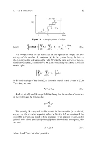
2.8.5 Poisson Arrivals During a Random Time Interval
Consider the number of arrivals (N) in a random time interval I. Assuming that
I is distributed with a probability density function A(t) and I is independent of
the Poisson process, then
P N k P N k I t A t dt
( ) ( | ) ( )
= = = =
∞
∫
0
But P N k I t
t
k
e
k
t
( | )
( )
!
= = = −
λ λ
Hence P N k
t
k
e A t dt
k
t
( )
( )
!
( )
= =
∞
−
∫
0
λ λ
last arrival next arrival
t = 0
t0
t
time
Figure 2.14 Conditional inter-arrival times](https://image.slidesharecdn.com/qtts-230925120453-047b3b23/85/QTTS-pdf-89-320.jpg)
![Taking the z-transform, we obtain
N z
t
k
e A t dt z
e
tz
k
k
k
t k
t
k
k
( )
( )
!
( )
( )
=
=
=
∞ ∞
−
∞
−
=
∞
∑ ∫
∫ ∑
0 0
0 0
λ
λ
λ
λ
!
!
( )
( )
)
)
A t dt
e A t dt
A z
z t
=
= −
∞
−( −
∫
0
λ λ
λ λ
*(
where A*(l − lz) is the Laplace transform of the arrival distribution evaluated
at the point (l − lz).
Example 2.5
Let us consider again the problem presented in Example 2.4. When this pas-
senger arrives at the station:
a) What is the probability that he will board a train in the next 5 minutes?
b) What is the probability that he will board a train in 5 to 9 minutes?
Solution
a) From Example 2.4, we have l = 1/10 = 0.1 min−1
, hence for a time period
of 5 minutes we have
λ
λ
λ
t
P train in
e t
k
e
t k
= × =
= = =
− −
5 0 1 0 5
0 5
0 5
0
0
0 5 0
. .
[
( )
!
( . )
!
.
and
min] .
.607
He will board a train if at least one train arrives in 5 minutes; hence
P[at least 1 train in 5 min] = 1 − P[0 train in 5 min]
= 0.393
b) He will need to wait from 5 to 9 minutes if no train arrives in the first 5
minutes and board a train if at least one train arrives in the time interval 5
to 9 minutes. From (a) we have
P[0 train in 5 min] = 0.607
PROPERTIES OF THE POISSON PROCESS 67](https://image.slidesharecdn.com/qtts-230925120453-047b3b23/85/QTTS-pdf-90-320.jpg)
![68 INTRODUCTION TO QUEUEING SYSTEMS
and P[at least 1 train in next 4 min] = 1 − P[0 train in next 4 min]
= − =
−
1
0 4
0
0 33
0 4 0
e .
( . )
!
.
Hence, P[0 train in 5 min at least 1 train in next 4 min]
= P[0 train in 5 min] × P[at least 1 train in next 4 min]
= 0.607 × 0.33 = 0.2
Example 2.6
Pure Aloha is a packet radio network, originated at the University of Hawaii,
that provides communication between a central computer and various remote
data terminals (nodes). When a node has a packet to send, it will transmit it
immediately. If the transmitted packet collides with other packets, the node
concerned will re-transmit it after a random delay t. Calculate the throughput
of this pure Aloha system.
Solution
For simplicity, let us make the following assumptions:
(i) The packet transmission time is one (one unit of measure).
(ii) The number of nodes is large, hence the total arrival of packets from all
nodes is Poisson with rate l.
(iii) The random delay t is exponentially distributed with density function
be−bt
, where b is the node’s retransmission attempt rate.
Giventheseassumptions,iftherearennodewaitingforthechanneltore-transmit
theirpackets,thenthetotalpacketarrivalpresentedtothechannelcanbeassumed
to be Poisson with rate (l + nb) and the throughput S is then given by
S = (l + nb)P[a successful transmission]
= (l + nb)Psucc
From Figure 2.15, we see that there will be no packet collision if there is
only one packet arrival within two units of time. Since the total arrival of
packets is assumed to be Poisson, we have
Psucc = e−2(l+nb)
and hence
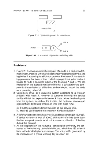
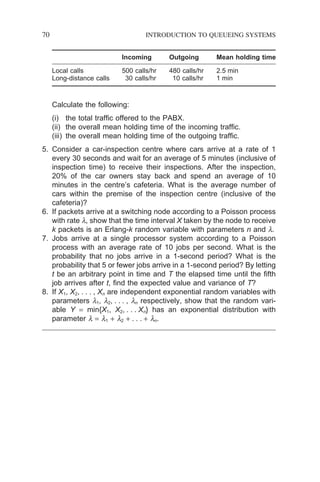
S = (l + nb)e−2(l+nb)](https://image.slidesharecdn.com/qtts-230925120453-047b3b23/85/QTTS-pdf-91-320.jpg)
![72 DISCRETE AND CONTINUOUS MARKOV PROCESSES
3.1 STOCHASTIC PROCESSES
Simply put, a stochastic process is a mathematical model for describing an
empirical process that changes with an index, which is usually the time in most
of the real-life processes, according to some probabilistic forces. More specifi-
cally, a stochastic process is a family of random variables {X(t), t ∈ T} defined
on some probability space and indexed by a parameter t{t ∈ T}, where t is
usually called the time parameter. The probability that X(t) takes on a value,
say i and that is P[X(t) = i], is the range of that probability space.
In our daily life we encounter many stochastic processes. For example, the
price Pst(t) of a particular stock counter listed on the Singapore stock exchange
as a function of time is a stochastic process. The fluctuations in Pst(t) through-
out the trading hours of the day can be deemed as being governed by probabi-
listic forces and hence a stochastic process. Another example will be the
number of customers calling at a bank as a function of time.
Basically, there are three parameters that characterize a stochastic process:
(1) State space
The values assumed by a random variable X(t) are called ‘states’ and the col-
lection of all possible values forms the ‘state space’ of the process. If X(t) = i
then we say the process is in state i. In the stock counter example, the state
space is the set of all prices of that particular counter throughout the day.
If the state space of a stochastic process is finite or at most countably infinite,
it is called a ‘discrete-state’ process, or commonly referred to as a stochastic
chain. In this case, the state space is often assumed to be the non-negative
integers {0, 1, 2, . . .}. The stock counter example mentioned above is a dis-
crete-state stochastic chain since the price fluctuates in steps of few cents or
dollars.
On the other hand, if the state space contains a finite or infinite interval of
the real numbers, then we have a ‘continuous-state’ process. At this juncture,
let us look at a few examples about the concept of ‘countable infinite’ without
going into the mathematics of set theory. For example, the set of positive
integer numbers {n} in the interval [a, b] is finite or countably infinite, whereas
the set of real numbers in the same interval [a, b] is infinite.
In the subsequent study of queueing theory, we are going to model the
number of customers in a queueing system at a particular time as a Markov
chain and the state represents the actual number of customers in the system.
Hence we will restrict our discussion to the discrete-space stochastic
processes.
(2) Index parameter
As mentioned above, the index is always taken to be the time parameter in the
context of applied stochastic processes. Similar to the state space, if a process
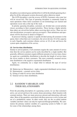
changes state at discrete or finite countable time instants, we have a](https://image.slidesharecdn.com/qtts-230925120453-047b3b23/85/QTTS-pdf-95-320.jpg)
![‘discrete (time) – parameter’ process. A discrete-parameter process is also
called a stochastic sequence. In this case, we usually write {Xk | k ∈ N = (0, 1,
2, . . .)} instead of the enclosed time parameter {X(t)}. Using the stock price
example again, if we are only interested in the closing price of that counter
then we have a stochastic sequence.
On the other hand, if a process changes state (or in the terminology of
Markov theory makes a ‘transition’) at any instant on the time axis, then we
have a ‘continuous (time) – parameter’ process. For example, the number of
arrivals of packets to a router during a certain time interval [a, b] is a continu-
ous-time stochastic chain because t ∈ [a, b] is a continuum.
Table 3.1 gives the classification of stochastic processes according to their
state space and time parameter.
(3) Statistical dependency
Statistical dependency of a stochastic process refers to the relationships between
one random variable and others in the same family. It is the main feature that
distinguishes one group of stochastic processes from another.
To study the statistical dependency of a stochastic process, it is necessary
to look at the nth order joint (cumulative) probability distribution which
describes the relationships among random variables in the same process. The
nth order joint distribution of the stochastic process is defined as
F x P X t x X t x
n n
( ) [ ( ) ( ) ]
= ≤ ≤
1 1,..., (3.1)
where
…
x x x xn
= ( )
1 2
, , ,
Any realization of a stochastic process is called a sample path. For example,
a sample path of tossing a coin n times is {head, tail, tail, head, . . . , head}.
Markov processes are stochastic processes which exhibit a particular kind
of dependency among the random variables. For a Markov process, its future
probabilistic development is dependent only on the most current state, and how
the process arrives at the current position is irrelevant to the future concern.
More will be said about this process later.
Table 3.1 Classifications of stochastic processes
Time Parameter State Space
Discrete Continuous
Discrete time discrete-time stochastic chain discrete-time stochastic process
Continuous time continuous-time stochastic
chain
continuous-time stochastic
process
STOCHASTIC PROCESSES 73](https://image.slidesharecdn.com/qtts-230925120453-047b3b23/85/QTTS-pdf-96-320.jpg)
![74 DISCRETE AND CONTINUOUS MARKOV PROCESSES
In the study of stochastic processes, we are generally interested in the prob-
ability that X(t) takes on a value i at some future time t, that is {P[X(t) = i]},
because precise knowledge cannot be had about the state of the process in
future times. We are also interested in the steady state probabilities if the prob-
ability converges.
Example 3.1
Let us denote the day-end closing price of a particular counter listed on the
Singapore stock exchange on day k as Xk. If we observed the following closing
prices from day k to day k + 3, then the following observed sequence {Xk} is
a stochastic sequence:
X X
X X
k k
k k
= =
= =
+
+ +
$ . $ .
$ . $ .
2 45 2 38
2 29 2 78
1
2 3
However, if we are interested in the fluctuations of prices during the trading
hours and assume that we have observed the following prices at the instants t1
t2 t3 t4, then the chain {X(t)} is a continuous-time stochastic chain:
X t X t
X t X t
( ) $ . ( ) $ .
( ) $ . ( ) $ .
1 2
3 4
2 38 2 39
2 40 2 36
= =
= =
3.2 DISCRETE-TIME MARKOV CHAINS
The discrete-time Markov chain is easier to conceptualize and it will pave the
way for our later introduction of the continuous Markov processes, which are
excellent models for the number of customers in a queueing system.
As mentioned in Section 3.1, a Markov process is a stochastic process which
exhibits a simple but very useful form of dependency among the random vari-
ables of the same family, namely the dependency that each random variable in
the family has a distribution that depends only on the immediate preceding
random variable. This particular type of dependency in a stochastic process
was first defined and investigated by the Russian mathematician Andrei A
Markov and hence the name Markov process, or Markov chain if the state space
is discrete. In the following sections we will be merely dealing with only the
discrete-state Markov processes; we will use Markov chain or process inter-
changeably without fear of confusion.
As an illustration to the idea of a Markov chain vs a stochastic process, let
us look at a coin tossing experiment. Firstly, let us define two random variables;
namely Xk = 1 (or 0) when the outcome of the kth trial is a ‘head’ (or tail), and
Yk = accumulated number of ‘heads’ so far. Assuming the system starts in state](https://image.slidesharecdn.com/qtts-230925120453-047b3b23/85/QTTS-pdf-97-320.jpg)
![Zero (Y0 = 0) and has the following sequence of the outcomes, as shown in
Table 3.2.
then we see that Xk defines a chain of random variables or in other words a
stochastic process, whereas Yk forms a Markov chain as its values depend only
on the cumulative outcomes and the preceding stage of the chain. That is
Y Y X
k k k
= +
−1 (3.2)
The probabilities that there are, say, five accumulated ‘heads’ at any stage
depends only on the number of ‘heads’ accumulated at the preceding stage (it
must be four or five) together with the fixed probability Xk on a given toss.
3.2.1 Definition of Discrete-time Markov Chains
Mathematically, a stochastic sequence {Xk, k ∈ T} is said to be a discrete-time
Markov chain if the following conditional probability holds for all i, j and k:
P X j X i X i X i X i P X j X i
k k k k k k
+ − − +
= = = = =
[ ] = = =
[ ]
1 0 0 1 1 1 1 1
, , , ,
… (3.3)
The above expression simply says that the (k + 1)th probability distribution
conditional on all preceding ones equals the (k + 1)th probability distribution
conditional on the kth; k = 0, 1, 2, . . . . In other words, the future probabilistic
development of the chain depends only on its current state (kth instant) and not
on how the chain has arrived at the current state. The past history has been
completely summarized in the specification of the current state and the system
has no memory of the past – a ‘memoryless’ chain. This ‘memoryless’ charac-
teristic is commonly known as the Markovian or Markov property.
The conditional probability at the right-hand side of Equation (3.3) is the
probability of the chain going from state i at time step k to state j at time step
k + 1 – the so-called (one-step) transitional probability. In general P[Xk+1 = j |
Xk = i] is a function of time and in Equation (3.3) depends on the time step k.
If the transitional probability does not vary with time, that is, it is invariant with
respect to time epoch, then the chain is known as a time-homogeneous Markov
chain. Using a short-hand notation, we write the conditional probability as
pij = P[Xk+1 = j | Xk = i]
Table 3.2 A sample sequence of Bernoulli trials
H H T T H T H H H T
Xk 1 1 0 0 1 0 1 1 1 0
Yk 1 2 2 2 3 3 4 5 6 6
DISCRETE-TIME MARKOV CHAINS 75](https://image.slidesharecdn.com/qtts-230925120453-047b3b23/85/QTTS-pdf-98-320.jpg)
![76 DISCRETE AND CONTINUOUS MARKOV PROCESSES
dropping the time index. Throughout this book, we will assume that all Markov
processes that we deal with are time homogeneous.
For notational convention, we usually denote the state space of a Markov
chain as {0, 1, 2, . . .}. When Xk = j, the chain is said to be in state j at time k
and we define the probability of finding the chain in this state using the new
notation:
π j
k
k
P X j
( )
[ ]
≡ = (3.4)
When a Markov chain moves from one state to another, we say the system
makes a ‘transition’. The graphical representation of these dynamic changes
of state, as shown in Figure 3.1, is known as the ‘state transition diagram’ or
‘transition diagram’ for short. In the diagram, the nodes represent states and
the directed arcs between nodes represent the one-step transition probabilities.
Those self-loops indicate the probabilities of remaining in the same state at the
next time instant. In the case of a discrete-time Markov chain, the transitions
between states can take place only at some integer time instants 0, 1, 2, . . . k,
whereas transitions in the continuous case may take place at any instant of
time.
As the system must transit to another state or remain in its present state at
the next time step, we have
j
ij ii
j i
ij
p p p
∑ ∑
= − =
≠
1 1
(3.5)
The conditional probability shown in Equation (3.3) expresses only the dyna-
mism (or movement) of the chain. To characterize a Markov chain completely,
it is necessary to specify the starting point of the chain, or in other words, the
initial probability distribution P[X0 = i] of the chain. Starting with the initial
state, it is in principle now possible to calculate the probabilities of finding the
chain in a particular state at a future time using the total probability theorem:
P X j P X j X i P X i p
k
i
k k k
i
i
k
ij
[ ] [ | ] [ ] ( )
+
=
∞
+
=
∞
= = = = = =
∑ ∑
1
0
1
0
π (3.6)
P
ii
P
ji
i j
P
jj
Pij
Figure 3.1 State transition diagram](https://image.slidesharecdn.com/qtts-230925120453-047b3b23/85/QTTS-pdf-99-320.jpg)
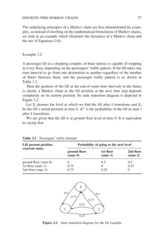
![78 DISCRETE AND CONTINUOUS MARKOV PROCESSES
p0
0 ≡ P(X0 = 0) = 1
p0
1 ≡ P(X0 = 1) = 0
p0
2 ≡ P(X0 = 2) = 0
Or in vector form
p̃(0)
= [p0
0, p0
1, p0
2] = [1, 0, 0]
(i) The probability of the lift’s position after 1st transition:
π
π
0
1
1
1 0 0
1
1
0
0
1 0 0 0 5 0 0 5 0
= =
= = = =
= × + × + × =
≡
∑
P X
P X X i P X i
P X
i
( )
( | ) ( )
. .
( 1
1
1 0 0
1
1
0 5
=
= = = =
=
∑
)
( | ) ( )
.
i
P X X i P X i
Similarly
p1
2 = P(X1 = 2) = 0.5
(ii) The probability of the lift’s position after 2nd transition:
π0
2
2
2 1 1
0
0
0 0 0 75 0 5 0 75 0 5
0
≡ =
= = = =
= × + × + ×
=
∑
P X
P X X i P X i
i
( )
( | ) ( )
. . . .
.7
75
and
p2
1 = P(X2 = 1) = 0.125
p2
2 = P(X2 = 2) = 0.125
From the above calculations, we see that we need only the probabilities of the
lift’s position after the 1st transition in order to calculate its probabilities after
the 2nd transition. That is to say that the future development of the process
depends only on its current position.](https://image.slidesharecdn.com/qtts-230925120453-047b3b23/85/QTTS-pdf-101-320.jpg)
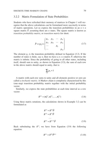
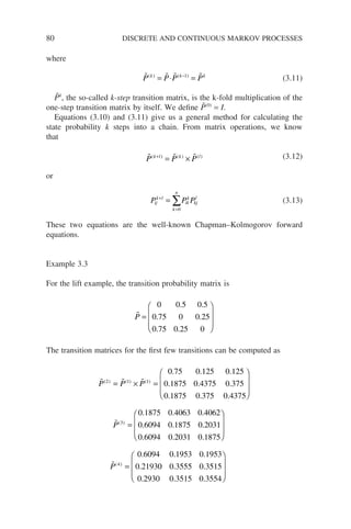
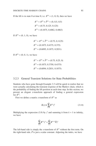
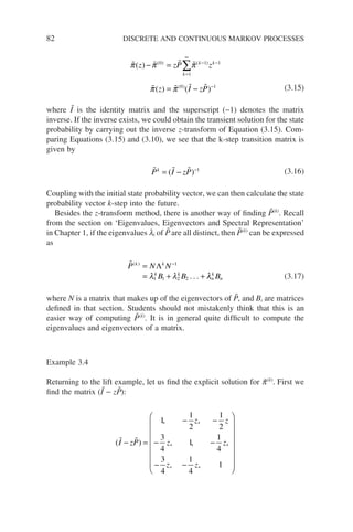

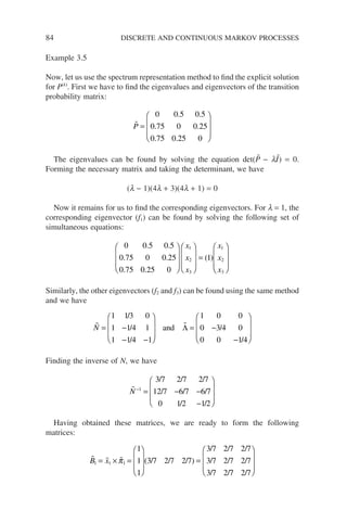
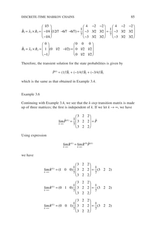
![86 DISCRETE AND CONTINUOUS MARKOV PROCESSES
We see that we always have the same final state probability vector when
k → ∞, regardless of the initial state probability if
π π
= ( )
→∞
lim k
k
exists.
3.2.4 Steady-state Behaviour of a Markov Chain
From Example 3.6, we see that the limiting value of
P P k
k
= ( )
→∞
lim is indepe-
dent of k and there exists a limiting value of the state probabilities
π π
= ( )
→∞
lim ,
k
k
which is independent of the initial probability vector.
We say these chains have steady states and p̃ is called the stationary prob-
ability or stationary distribution. The stationary probability can be calculated
from Equation (3.9) as
lim lim
k
k
k
k
P P
→∞ →∞
−
= → =
π π π π
( ) ( )
1
(3.18)
For most of the physical phenomena and under very general conditions that
are of interest to us, limiting values always exist. We will state a theorem
without proof but clarify some of the terms used in the theorem
subsequently.
Theorem 3.1
A discrete Markov chain {Xk} that is irreducible, aperiodic and time-homoge-
neous is said to be ergodic. For an ergodic Markov chain, the limiting
probabilities:
π π
π π
j
k
j
k
k
k
k
k
P X j j
= = = =
=
→∞ →∞
→∞
lim lim , , . . .
lim matrix
( )
( )
[ ]
(
0 1
n
notation)
always exist and are independent of the initial state probability distribution.
The stationary probabilities pj are uniquely determined through the following
equations:
j
j
∑ =
π 1 (3.19)
π π
j
i
i ij
P
= ∑ (3.20)
Expressions (3.19) and (3.20) can be formulated using matrix operations as
follows:](https://image.slidesharecdn.com/qtts-230925120453-047b3b23/85/QTTS-pdf-109-320.jpg)
![p̃ ·ẽ = 1
p̃ = p̃ ·P̃
where ẽ is a 1 × n row vector with all entries equal to one.
To solve these two matrix equations, we first define a n × n matrix Ũ with
all entries equal to one, then the first equation can be rewritten as p̃ ·Ũ = ẽ.
Students should note that these two matrices, Ũ or ẽ, have the summation
property. Any matrix, say à = [aij], multiplied by Ũ or ẽ will give rise to a
matrix in which every entry in a row is the same and is the sum of the corre-
sponding row in Ã. For example:
a a
a a
a a a a
a a a a
11 12
21 22
11 12 11 12
21 22 21 22
1 1
1 1
=
+ +
+ +
Adding the two equations together, we have
π( )
P U I e
+ − = (3.21)
We will postpone our discussion of some terms, for example, aperiodic and
irreducible, used in the theorem to the next section and instead look at how we
could use this theorem to calculate the steady-state probabilities of a Markov
chain.
Example 3.7
Continuing with the lift example, the transition probabilities are given by
P pij
= =
( )
/ /
/ /
/ /
0 1 2 1 2
3 4 0 1 4
3 4 1 4 0
and steady state probabilities p̃ = [p0, p1, p2]. Using Equation (3.18) and
expanding it, we have
π π π π
π π π π
π π π π
0 0 1 2
1 0 1 2
2 0 1 2
0
3
4
3
4
1
2
0
1
4
1
2
1
4
0
= + +
= + +
= + +
DISCRETE-TIME MARKOV CHAINS 87](https://image.slidesharecdn.com/qtts-230925120453-047b3b23/85/QTTS-pdf-110-320.jpg)
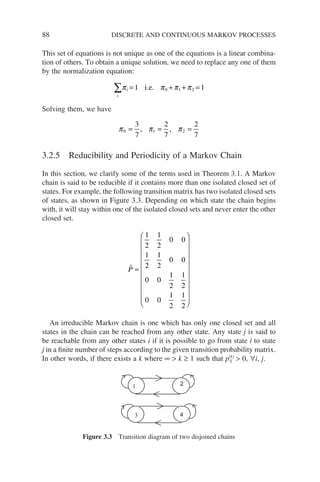

![90 DISCRETE AND CONTINUOUS MARKOV PROCESSES
Example 3.9
The two simplest examples of periodic Markov chain are shown below. If we
assume that the initial position of these two chains is state 1, then the first chain
will always go back to state 1 after two transitions and the second chain after
three transitions (Figure 3.5).
The transition probability matrices for these two Markov chains are
P P
1 2
0 1
1 0
0 1 0
0 0 1
1 0 0
=
and
respectively. If we compute the k-step transition probability matrices, we
have
P P P
P P P
1 1
3
1
5
2 2
4
2
7
0 1
1 0
0 1 0
0 0
= = = =
= = = =
( ) ( )
( ) ( )
. . .
. . . 1
1
1 0 0
We see that these two Markov chains have periods 2 and 3, respectively.
Note that these two chains still have a stationary probability distribution though
they are periodic in nature. Students can verify that the stationary probabilities
are given as
p̃ = [0.5 0.5] two-state chain
π = [ ]
1 3 1 3 1 3 three-state chain
3.2.6 Sojourn Times of a Discrete-time Markov Chain
Sojourn time of a discrete-time Markov chain in a given state, say i, refers to
the number of time units it spends in that state. We will restrict our discussion
to the homogeneous Markov chains here.
2
2
1 3
1
Figure 3.5 Periodic Markov chain](https://image.slidesharecdn.com/qtts-230925120453-047b3b23/85/QTTS-pdf-113-320.jpg)
![Assuming the Markov chain has just entered state i, the probability of it
staying in this state at the next time step is given by p p
ij ij
i j
= −
≠
∑
1 . If it stays
in this state, again the probability of it staying in that state at the next time step
is also pii. Hence, we see that the time a Markov chain stays in a state i, sojourn
time Ri, is a geometrically distributed random variable with pmf:
P R k p p k
i ii ii
k
[ ] ( )
= = − ∀ =
−
1 1 2 3
1
, , , ,... (3.22)
And the expected sojourn time is given by
E R
p
i
ii
[ ] =
−
1
1
The previous result of the sojourn time is in line with the memoryless prop-
erty of a Markov chain. The geometric distribution is the only discrete pro-
bability distribution that possesses such a memoryless property. Exponential
distribution is the continuous version that also possesses such a property and
we will show later that the sojourn times of a continuous-time Markov chain
is exponentially distributed.
3.3 CONTINUOUS-TIME MARKOV CHAINS
Having discussed the discrete-time Markov chain, we are now ready to look
at its continuous-time counterpart. Conceptually, there is no difference between
these two classes of Markov chain; the past history of the chain is still being
summarized in its present state and its future development can be inferred from
there. In fact, we can think of the continuous-time Markov chain as being the
limiting case of the discrete type.
However, there is a difference in mathematical formulation. In a continuous
Markov chain, since transitions can take place at any instant of a time contin-
uum, it is necessary now to specify how long a process has stayed in a particular
state before a transition take place.
In some literature, the term ‘Markov process’ is also used to refer to a con-
tinuous-time Markov chain. We use that term occasionally in subsequent
chapters.
3.3.1 Definition of Continuous-time Markov Chains
The definition of a continuous-time Markov chain parallels that of a discrete-
time Markov chain conceptually. It is a stochastic process {X(t)} in which the
future probabilistic development of the process depends only on its present
CONTINUOUS-TIME MARKOV CHAINS 91](https://image.slidesharecdn.com/qtts-230925120453-047b3b23/85/QTTS-pdf-114-320.jpg)
![92 DISCRETE AND CONTINUOUS MARKOV PROCESSES
state and not on its past history. Mathematically, the process should satisfy the
following conditional probability relationships for t1 t2 . . . tk:
P X t j X t i X t t X t i P X t j X t
k k k k
[ ( ) | ( ) ( ) ( ) ] [ ( ) | (
+ +
= = = = = =
1 1 1 2 2 1
, , . . . k
k k
i
) ]
=
(3.23)
From the early discussion, we know that in the treatment of continuous-time
Markov chains we need to specify a transition scheme by which the system
goes from one state to another. The transition probability alone is not sufficient
to completely characterize the process. Instead of dwelling on its formal theo-
retical basics which can be quite involved, we will take the following definition
as the point of departure for our subsequent discussions and develop the neces-
sary probability distribution. And again, we will focus our attention on the
homogeneous case.
Definition 3.1
For a continuous Markov chain which is currently in state i, the probability
that the chain will leave state i and go to state j(j ≠ i) in the next infinitesimal
amount of time ∆t, no matter how long the chain has been in state i, is
pij(t, t + ∆t) = qij∆t
where qij is the instantaneous transition rate of leaving state i for state j. In
general, qij is a function of t. To simply the discussion, we assume that qij is
independent of time; in other words, we are dealing with a homogeneous
Markov chain. The total instantaneous transition rate at which the chain leaves
state i is, therefore,
j i
ij
q
≠
∑ .
3.3.2 Sojourn Times of a Continuous-time Markov Chains
Analogous to the discrete-time Markov chain, the sojourn times of a continu-
ous-time Markov chain is the time the chain spends in a particular state. From
the earlier discussion of Markov chains, we know that the future probabilistic
development of a chain is only related to the past history through its current
position. Thus, the sojourn times of a Markov chain must be ‘memoryless’ and
are exponentially distributed, as exponential distribution is the only continuous
probability distribution that exhibits such a memoryless property.
We shall demonstrate that the sojourn times of a continuous-time Markov
chain are indeed exponentially distributed using the above definition. We
assume the chain has just entered state i, and will remain in that during an
interval [0, t].](https://image.slidesharecdn.com/qtts-230925120453-047b3b23/85/QTTS-pdf-115-320.jpg)
![Let ti be the random variable that denotes the time spent in state i. If we
divide the time t into k equal intervals of ∆t, such that k∆t = t, then for the
sojourn time ti to be greater than t, there should not be any transition in any
of these ∆t intervals. From the above definition, we know that the probability
of not having a transition in a time interval ∆t is
1−
≠
∑
j i
ij
q t
∆
Therefore, the probability that the sojourn is greater than t
P t q t
q
t
k
i
k
j i
ij
k
k
j i
ij
k
[ ]
τ = −
= −
=
→∞
≠
→∞
≠
∑
∑
lim
lim
1
1
∆
e
e q t
i
−
(3.24)
where q q
i
j i
ij
= −
≠
∑ . Hence, the sojourn time between transitions is given by
P t P t e
i i
q t
i
[ ] [ ]
τ τ
≤ = − = − −
1 1 (3.25)
which is an exponential distribution.
3.3.3 State Probability Distribution
We will now turn our attention to the probability of finding the chain in a par-
ticular state – state probability. As usual, we define pj(t) = P[X(t) = j] and
consider the probability change in an infinitesimal amount of time ∆t:
π π π
j
i j
i ij j
k j
jk
t t t q t t q t
( ) ( ) ( )
+ = + −
≠ ≠
∑ ∑
∆ ∆ ∆
1 (3.26)
The first term on the right is the probability that the chain is in state i at time
t and makes a transition to state j in ∆t. The second term is the probability that
the chain is in state j and does not make a transition to any other states in ∆t.
Rearranging terms, dividing Equation (3.20) by ∆t and taking limits, we have
d
dt
t q q
j
i j
i ij j
k j
jk
π π π
( ) = −
≠ ≠
∑ ∑ (3.27)
CONTINUOUS-TIME MARKOV CHAINS 93](https://image.slidesharecdn.com/qtts-230925120453-047b3b23/85/QTTS-pdf-116-320.jpg)
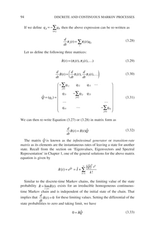
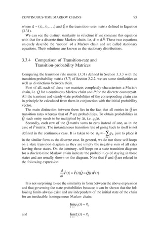
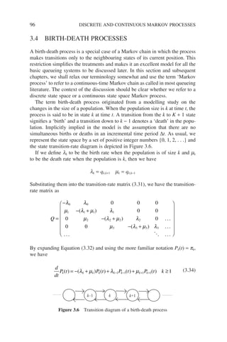
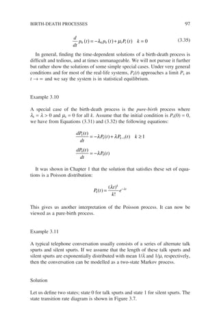
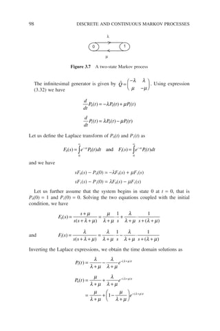
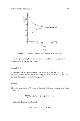
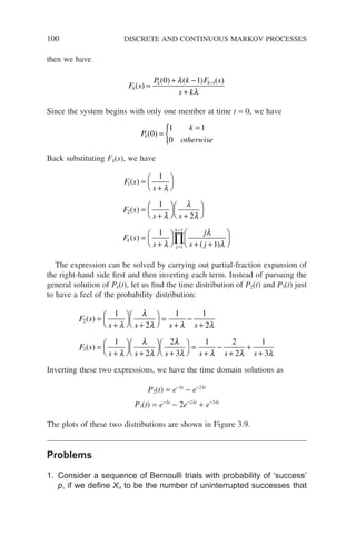
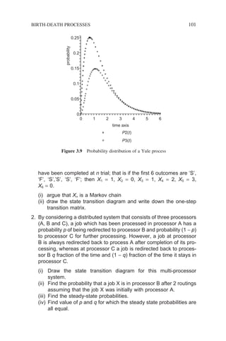
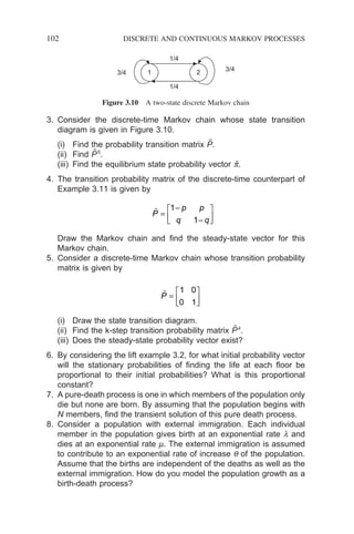
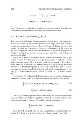
![( )
λ µ λ µ
+ = +
− +
P P P
k k k
1 1 (4.3)
µ λ
P P
1 0
= (4.4)
Equation (4.3) is a recursive expression and we shall solve it using z-trans-
form. Multiplying the whole equation by zk
and summing from one to infinity,
we have
k
k
k
k
k
k
k
k
k
P z P z P z
=
∞
=
∞
−
=
∞
+
∑ ∑ ∑
+ = +
1 1
1
1
1
( )
λ µ λ µ
( )[ ( ) ] ( ) [ ( ) ]
λ µ λ
µ
+ − = + − −
P z P zP z
z
P z P z P
0 1 0
Coupled with the boundary conditions of Equation (4.4), P P
1 0
=
λ
µ
, we have
( ) ( ) [ ( ) ] ( )
( )
( )
( )
λ µ µ
µ
λ
µ
λ λ µ µ
+ − = − +
=
−
− + +
=
P z P
z
P z P zP z
P z
P z
z z
0 0
0
2
1 P
P z
z z
P
z
P
z
0
0
0
1
1
1
1
1
µ
λ µ
λ
µ
ρ
ρ λ µ
( )
( )( )
/
−
− −
=
−
=
−
=
where (4.5)
To evaluate P0, we use the normalization condition
k
k
p
=
∞
∑ =
0
1, which is
equivalent to P(z)
z=1 = 1. Setting z = 1 and P(z) = 1, we have
P0 1 1
= − = −
λ
µ
ρ (4.6)
Hence we arrive at
P z
z
( ) =
−
−
1
1
ρ
ρ
(4.7)
and
CLASSICAL M/M/1 QUEUE 105](https://image.slidesharecdn.com/qtts-230925120453-047b3b23/85/QTTS-pdf-128-320.jpg)
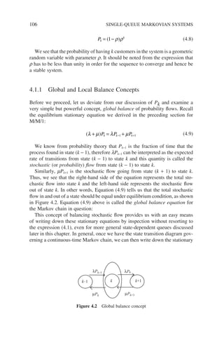
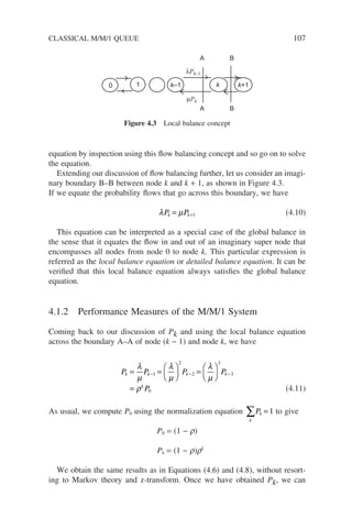
![108 SINGLE-QUEUE MARKOVIAN SYSTEMS
proceed to find other performance measures using Little’s theorem. Students
should note that this local balance concept offers a simpler expression
for computing Pk and this should be the preferred approach as far as
possible:
(i) The probability of having n or more customers in the system is given by
P N n P
k n
k
k n
k
k
k
k
n
k
[ ]
( )
( )
(
≥ =
= −
= − −
=
=
∞
=
∞
=
∞
=
−
∑
∑
∑ ∑
1
1
0 0
1
ρ ρ
ρ ρ ρ
1
1
1
1
1
1
−
−
−
−
−
=
ρ
ρ
ρ
ρ
ρ
)
n
n
(4.12)
(ii) The average number of customers N in the system in steady state is then
given by
N kP k
k
k
k
k
k
k
k
= = −
( )
= −
=
−
=
−
=
∞
=
∞
=
∞
−
∑ ∑
∑
0 0
0
1
1
1
1
ρ ρ
ρ ρ ρ
ρ
ρ
λ
µ λ
( )
(4.13)
and the variance of N can be calculated as
σ
ρ
ρ
N
k
k
k N p
2
0
2
2
1
= − =
−
=
∞
∑( )
( )
(4.14)
Figure 4.4 shows the average number of customers as a function of utiliza-
tion r. As the utilization (load) approaches the full capacity of the system
(r = 1), the number of customers grows rapidly without limit and the system
becomes unstable. Again, we see that for the system to be stable, the condition
is r 1.
This is a significant result for a single isolated queueing system and is the
basis of the ‘two-third’ design rule. In practice, we usually design a shared](https://image.slidesharecdn.com/qtts-230925120453-047b3b23/85/QTTS-pdf-131-320.jpg)
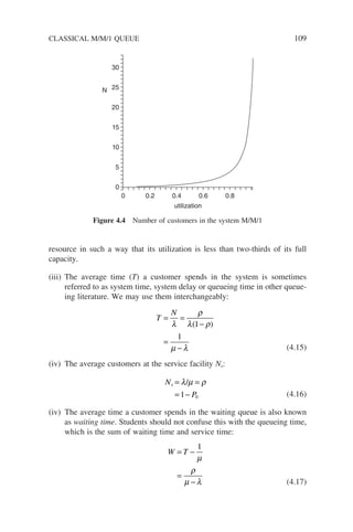
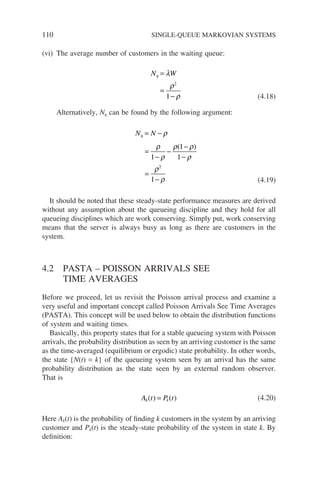
![A t P N t k An arrival at time t
P N t k An arrival at time t
k( ) [ ( ) | ]
[ ( )
≡ =
=
= , ]
]
[ ]
[ | ( ) ] [ ( ) ]
P An arrival at time t
P An arrival at time t N t k P N t k
=
= ⋅ =
P
P An arrival at time t
[ ]
However, we know that the event of an arrival at time t is independent of
the process {N(t) = k} because of the memoryless property of Poisson process.
That is
P[An arrival at time t N(t) = k] = P[An arrival at time t]
Therefore, substituting in the preceding expression, we obtain
A t P N t k P t
k k
( ) [ ( ) ] ( )
= = = (4.21)
In the limit of t → ∞, we have
A P
k k
= (4.22)
4.3 M/M/1 SYSTEM TIME (DELAY) DISTRIBUTION
In previous sections, we obtained several performance measures of an M/M/1
queue, so we are now in a position to predict the long-range averages of this
queue. However, we are still unable to say anything about the probability that
a customer will spend up to 3 minutes in the system or answer any questions
on that aspect. To address them, we need to examine the actual probability
distribution of both the system time and waiting time. Let us define the system-
time density function as
f t
d
dt
P T t
T( ) [ ]
=
Students should note that the probability distributions (or density functions)
of system time or waiting time depend very much on the actual service disci-
pline used, although the steady state performance measures are independent of
the service discipline.
We assume here that FCFS discipline is used and focus our attention on the
arrival of customer i. The system time of this customer will be the sum of his/
her service time and the service times of those customers (say k of them) ahead
M/M/1 SYSTEM TIME (DELAY) DISTRIBUTION 111](https://image.slidesharecdn.com/qtts-230925120453-047b3b23/85/QTTS-pdf-134-320.jpg)
![112 SINGLE-QUEUE MARKOVIAN SYSTEMS
of him/her if the system is not empty when he/she arrives. Otherwise, his/her
system time will be just his/her own service time. That is
T
x x x x k
x k
i k
i
=
+ + + + ≥
=
{ 1 2 1
0
...
(4.23)
Owing to the memoryless property of exponential service times, the
remaining service time needed to finish serving the customer currently in
service is still exponentially distributed. Hence the density function of T is
simply the convolution of all the service times which are all exponentially
distributed.
Using Laplace transform, the conditional system-time density function is
L f t k
s
k
T
k
[ ( | )] =
+
=
+
µ
µ
1
0 1 2
, , , . . . (4.24)
Earlier we obtained Pk = (1 − r)rk
, hence the Laplace transform of the
unconditional probability density function can be obtained using the total prob-
ability theorem:
L f t
s
s
T
k
k
k
[ ( )] ( )
( )
=
+
−
=
−
+ −
=
∞ +
∑
0
1
1
µ
µ
ρ ρ
µ λ
µ λ
(4.25)
Inverting the above expression, we have
f t e t
T
t
( ) ( ) ( )
= −
− −
µ λ µ λ
, 0 (4.26)
and the cumulative distribution function FT(t) is
F t P T t e
T
t
( ) [ ] ( )
= ≤ = − − −
1 µ λ
(4.27)
At this juncture, it is important to point out that the above expression was
actually derived with respect to an arriving customer. However, owing to the
PASTA property of a Poisson arrival process, these probability distributions
are the same as the long-range time averages or, in other words, distributions
seen by a random observer.
Once the density function of system time is found, the density function of
waiting time fw(t) can be found by considering:
T w x
= + (4.28)](https://image.slidesharecdn.com/qtts-230925120453-047b3b23/85/QTTS-pdf-135-320.jpg)
![Taking Laplace transform, we have
µ λ
µ λ
µ
µ
µ ρ
µ λ
ρ
λ
−
+ −
=
+
=
+ −
+ −
= − +
s
L f s
s
L f s
s
s
w
w
( )
[ ( )]
( ( )]
( )( )
( )
( )
(
1
1
1
1−
+ −
ρ
µ λ
)
( )
s
(4.29)
Inverting
f t t e
w
t
( ) ( ) ( ) ( ) ( )
= − + − − −
1 1
ρ δ λ ρ µ λ
(4.30)
where d(t) is the impulse function or Dirac delta function.
Integrating we have the waiting time cumulative distribution function
Fw(t):
F t e
w
t
( ) ( )
= − − −
1 ρ µ λ
(4.31)
Example 4.1
At a neighhourhood polyclinic, patients arrive according to a Poisson process
with an average inter-arrival time of 18 minutes. These patients are given a
queue number upon arrival and will be seen, by the only doctor manning the
clinic, according to their queue number. The length of a typical consultation
session is found from historical data to be exponentially distributed with a mean
of 7 minutes:
(i) What is the probability that a patient has to wait to see the doctor?
(ii) What is the average number of patients waiting to see the doctor?
(iii) What is the probability that there are more than 5 patients in the clinic,
including the one in consultation with the doctor?
(iv) What is the probability that a patient would have to wait more than 10
minutes for this consultation?
(v) The polyclinic will employ an additional doctor if the average waiting time
of a patient is at least 7 minutes before seeing the doctor. By how much
must the arrival rate increase in order to justify the additional doctor?
Solution
Assuming the clinic is sufficiently large to accommodate a large number of
patients, the situation can be modelled as an M/M/1 queue. Given the following
parameters:
M/M/1 SYSTEM TIME (DELAY) DISTRIBUTION 113](https://image.slidesharecdn.com/qtts-230925120453-047b3b23/85/QTTS-pdf-136-320.jpg)
![114 SINGLE-QUEUE MARKOVIAN SYSTEMS
l = 1/18 person/min and m = 1/7 person/min
We have r = 7/18:
(i) P[patient has to wait] = r = 1 − P0 = 7/18
(ii) The waiting-queue length Nq = r2
/(1 − r) = 49/198
(iii) P[N ≥ 5] = r5
= 0.0089
(iv) Since P[waitingtime ≤ 10] = 1 − re−m(1−r)t
,
P e
[ ] .
/ /
queueing time = =
− −
( )×
10
7
18
0 162
1 7 1 7 18 10
(v) Let the new arrival rate be l′
then
7
1
7
7
1
14
′
− ′
≥ ⇒ ′ =
λ
λ
λ person/min person/min.
Example 4.2
Variable-length data packets arrive at a communication node according to
a Poisson process with an average rate of 10 packets per second. The
single outgoing communications link is operating at a transmission rate of
64 kbits per second. As a first-cut approximation, the packet length can
be assumed to be exponentially distributed with an average length of 480
characters in 8-bit ASCII format. Calculate the principal performance mea-
sures of this communication link assuming that it has a very large input
buffer. What is the probability that 6 or more packets are waiting to be
transmitted?
Solution
Again the situation can be modelled as an M/M/1 with the communication link
being the server.
The average service time:
x =
×
=
480 8
64000
0 06
. s
and the arrival rate
l = 10 packets/second
thus](https://image.slidesharecdn.com/qtts-230925120453-047b3b23/85/QTTS-pdf-137-320.jpg)
![r = lx̄ = 10 × 0.06 = 0.6
The parameters of interest can be calculated easily as:
N N
T W
q
=
−
= =
−
=
=
−
=
ρ
ρ
ρ
ρ
µ λ
1
3
2 1
9
10
1 1
2
2
packets and packets
seconds and =
=
−
=
≥
=
−
x
P
ρ
ρ
1
7
1
3
10
7
seconds
number of packets in the system
[ ]
=
=
=
( . )
.
0 6
0 028
7
Example 4.3
In an ATM network, two types of packets, namely voice packets and data
packets, arrive at a single channel transmission link. The voice packets are
always accepted into the buffer for transmission but the data packets are only
accepted when the total number of packets in the system is less than N.
Find the steady-state probability mass function of having k packets in the
system if both packet streams are Poisson with rates l1 and l2, respectively.
You may assume that all packets have exponentially distributed lengths and
are transmitted at an average rate m.
Solution
Using local balance concept (Figure 4.5), we obtain the following equations:
P
P k N
P k N
k
k
k
=
+
≤
−
−
λ λ
µ
λ
µ
1 2
1
1
1
0 1 N+1 N+2
λ
1+ λ
2
N
λ
1
+ λ
2 λ1 λ1
µ µ µ µ µ µ
λ1
Figure 4.5 Transition diagram for Example 4.3
M/M/1 SYSTEM TIME (DELAY) DISTRIBUTION 115](https://image.slidesharecdn.com/qtts-230925120453-047b3b23/85/QTTS-pdf-138-320.jpg)
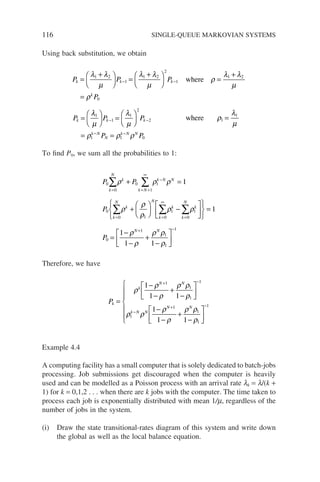
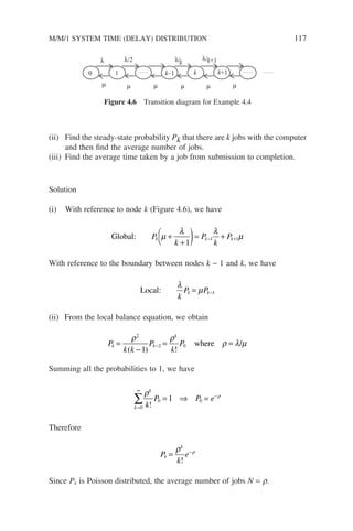
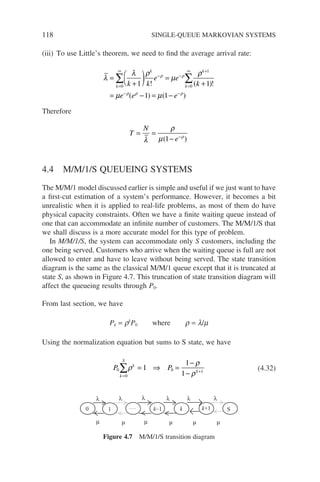
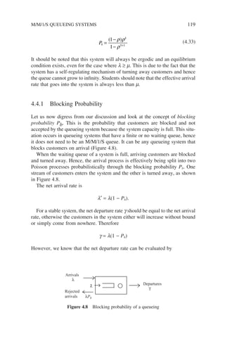
![(ii) The average number of customers in the system is given by
N kP
k
k
k
S
k
k
S
S
k
S
k
s
=
=
−
−
=
−
−
=
=
+
+
=
∑
∑
∑
0
1
1
1
1
1
1
1
1
ρ
ρ
ρ
ρ
ρ
ρ ρk
k
S
k
s
k
S
S
d
d
S
−
+
=
+
+
=
−
−
=
−
−
+
−
=
−
−
∑
1
1
1
1
1
1
1
1
1
1
1
ρ
ρ
ρ
ρ
ρ
ρ
ρ
ρ
ρ
ρ
ρ
( )
ρ
ρ
ρ
1
1
−
+
( )
S PS (4.37)
Again, for r = 1, the expression has to be evaluated by L’Hopital’s rule
and we have
N
S
=
2
(4.38)
(iii) The average number of customers at the service facility:
N P k E N k P k E N N
P
P
s s s
S
= = = +
= −
= −
[ ] [ | ] [ ] [ | ]
( )
0 0 0 0
1
1
0
ρ (4.39)
(iv) The average number of customers in the waiting queue:
N N N
S
P
q s S
= − =
−
−
+
−
ρ
ρ
ρ ρ
ρ
2
1 1
( )
(4.40)
(v) The average time spent in the system and in the waiting queue.
Since customers are blocked when there are S customers in the system,
the effective arrival rate of customers admitted into the system is
′ = −
λ λ( )
1 Ps (4.41)
and the T and W can be computed as
T
N S S
S
=
′
=
−
−
−
+
+
λ µ λ
ρ
λ µρ
1 1
1
(4.42)
M/M/1/S QUEUEING SYSTEMS 121](https://image.slidesharecdn.com/qtts-230925120453-047b3b23/85/QTTS-pdf-144-320.jpg)
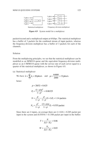
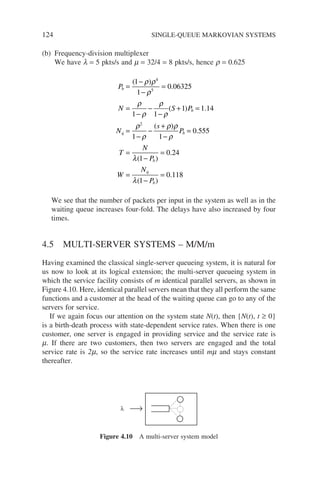
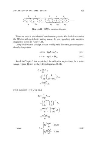
![126 SINGLE-QUEUE MARKOVIAN SYSTEMS
Using the normalization condition ∑ =
Pk 1, we obtain
P
m
k
m
m
P
m
k
m
k
m k
k m
m k
k
m k
0
0
1
0
0
1
1
=
−
=
∞
=
−
∑ ∑
∑
+
=
= +
( )
! !
( )
!
( )
ρ ρ
ρ ρ m
m
k m
k m
k
m k m
m
m
k
m
m
!
( )
!
( )
!( )
=
∞
−
−
=
− −
∑
∑
= +
−
ρ
ρ ρ
ρ
1
0
1 1
1
(4.47)
Similar to the M/M/1 case, r = l/mm 1 is the condition for this system to be
stable.
4.5.1 Performance Measures of M/M/m Systems
Once we have obtained Pk, as usual we can proceed to find other parameters.
However, we usually express the performance measures of M/M/m systems in
terms of a probability called delay probability or queueing probability, because
this probability is widely used in designing telephony systems. It corresponds
to the situation in classical telephony where no trunk is available for an arriving
call. Its tabulated results are readily available and hence other parameters can
be easily calculated.
(i) The probability of delay
This is the probability that an arriving customer finds all servers busy and
is forced to wait in the queue. This situation occurs when there are more
than m customers in the system, hence we have
P P delay P
P m
m
P m
m
d
k m
k
o
m
k m
k m
m
= =
=
=
−
=
∞
=
∞
−
∑
∑
[ ]
( )
!
( )
!( )
ρ
ρ
ρ
ρ
0
1 (4.48)
This probability is often referred to as the Erlang C formula or the Erlang
Delay formula and is often written as C(l/m, m). Most of the parameters
of interest can be expressed in terms of this probability.
(ii) As the probability mass function Pk consists of two functions, it is easier
to first find Nq, the number of customers waiting in the queue, instead of
N so that the discontinuity in pmf can be avoided:](https://image.slidesharecdn.com/qtts-230925120453-047b3b23/85/QTTS-pdf-149-320.jpg)
![N kP P
m
m
k
P
m
m
P
m
q
k
m k
m
k
k
m
d
= =
=
−
=
−
=
=
∞
+
=
∞
∑ ∑
0
0
0
0 2
1
1
( )
!
( )
! ( )
ρ
ρ
ρ ρ
ρ
ρ
ρ
λ
µ
µ λ
−
Pd (4.49)
(iii) The time spent in the waiting queue:
W
N
m
P
q
d
= =
−
λ µ λ
1
(4.50)
(iv) The time spends in the queueing system:
T W
P
m
d
= + =
−
+
1 1
µ µ λ µ
(4.51)
(v) The number of customers in the queueing system:
N T P m
d
= =
−
+
λ
ρ
ρ
ρ
1
(4.52)
4.5.2 Waiting Time Distribution of M/M/m
Parallel to the M/M/1 case, we will continue with the examination of the
waiting time distribution in this section. Again, we are going to make use of
the PASTA concept to derive the function. Let us focus our attention on an
arriving customer i to the system. He/her may find k customers waiting in the
queue upon arrival, meaning there are n = (k + m) customers in the system.
He/she may also find no customers waiting in the queue, meaning the total
number of customers is n ≤ m − 1.
We denote the waiting time of this customers i as w, and its density function
as fw(t) and cumulative probability function Fw(t); then we have
F t P w t
P w t no waiting P w t k
w( ) [ ]
[ ] [ ]
=
= + ≥
, , 0 (4.53)
Let us examine each individual term on the right-hand side of the expression.
The first term is simply the probability of having n ≤ m − 1 customers in the
system, hence no waiting:
MULTI-SERVER SYSTEMS – M/M/m 127](https://image.slidesharecdn.com/qtts-230925120453-047b3b23/85/QTTS-pdf-150-320.jpg)
![128 SINGLE-QUEUE MARKOVIAN SYSTEMS
P w t no waiting P n m
P P
m
k
n
m
n
n
m k
[ ] [ ]
( )
!
= ≤ −
= =
=
−
=
−
∑ ∑
, 1
0
1
0
0
1
ρ (4.54)
But, we have from Equation (4.47):
P
m
k
m
m
k
m k m
0
0
1 1
1
= +
−
=
− −
∑
( )
!
( )
!( )
ρ ρ
ρ
P
m
k
P m
m
k
m k m
0
0
1
0
1
1
=
−
∑ = −
−
( )
!
( )
!( )
ρ ρ
ρ
Hence
P w t no waiting
P m
m
m
[ ]
( )
!( )
= −
−
, 1
1
0 ρ
ρ
(4.55)
The second term depicts the situation where customer i has to wait in the
queue. His/her waiting time is simply the sum of the service time xj (j =
1, . . . k) of those k customers in the queue as well as the service time x of those
customers currently in service. That is
w = x + x1 + x2 + . . . + xk
The service times are all exponentially distributed with a rate mm, as there
are m servers. Therefore the density function of w is simply the convolution of
these service times, and in Laplace transform domain, the multiplication of
them. Thus we have
L f t k
m
s m
k
w
k
{ ( | )} =
+
= ∞
+
µ
µ
1
0 1
, , , . . . ,
and
L f t
m
s m
P
m
s m
P
w
k
k
k m
k
k
{ ( )} =
+
⋅ =
+
⋅
=
∞ +
+
=
∞ +
∑ ∑
0
1
0
1
0
µ
µ
µ
µ
m
m
m
P
m
m
m
s m
m
s m
P
m
m
k m
m
k
k
k
!
( )
!
(
ρ
ρ µ
µ
µ
µ
ρ
ρ
+
=
∞
=
+
+
⋅
=
∑
0
0
0
)
)
!
( )
!
m
m
m
m
s m
s m
s m
P
m
m
m
s m
µ
µ
µ
µ λ
ρ µ
µ λ
+
+
+ −
=
+ −
0 (4.56)](https://image.slidesharecdn.com/qtts-230925120453-047b3b23/85/QTTS-pdf-151-320.jpg)
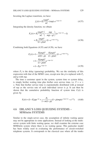
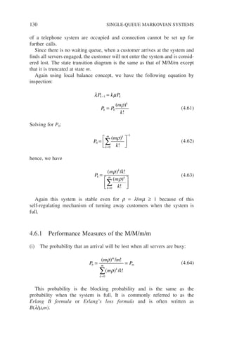
![(ii) The number of customers in the queueing system:
N kP k P
m
k
m P
m
k
m
m
k
m
k
k
m k
k
m k
k
m
= = ⋅ =
=
= = =
−
=
∑ ∑ ∑
∑
0 1
0
0
1
0
0
( )
!
( )
( )
!
(
ρ
ρ
ρ
ρ
ρ
ρ ρ
ρ
ρ ρ
)
!
( )
!
( )
!
( )( ) ( )
k m
i
m i m b
k
m
m
m
i
m P m P
−
= − = −
=
∑
0
1 1 (4.65)
(iii) The system time and other parameters
Since there is no waiting, the system time (or delay) is the same as service time
and has the same distribution:
T =1/µ (4.66)
F t P T t e
T
t
( ) [ ]
= ≤ = − −
1 µ
(4.67)
N W
q = =
0 0
and (4 68)
4.7 ENGSET’S LOSS SYSTEMS
So far, we have always assumed that the size of the arriving customers or cus-
tomer population is infinite, and hence the rate of arrivals is not affected by
the number of customers already in the system. In this section, we will look at
a case where the customer population is finite and see how it can be adapted
to the birth-death process.
Engset’s loss system is a ‘finite population’ version of Erlang’s loss
system. This is a good model for a time-sharing computer system with a
group of fully-occupied video terminals. The jobs generated by each video
terminal are assumed to be a Poisson process with rate l. When a user at
a video terminal has submitted a job, he is assumed to be waiting for the
reply (answer) from the central CPU, and hence the total jobs’ arrival rate
is reduced.
In this mode, we again have m identical parallel servers and no
waiting queue. However, we now have a finite population (C) of arriv-
ing customers instead of infinite population of customers, as shown in
Figure 4.12.
To reflect the effect of the reduced arrival rate due to those customers already
arrived at the system, the following parameters for the birth-death process are
selected. The state transition diagram is shown in Figure 4.13.
ENGSET’S LOSS SYSTEMS 131](https://image.slidesharecdn.com/qtts-230925120453-047b3b23/85/QTTS-pdf-154-320.jpg)
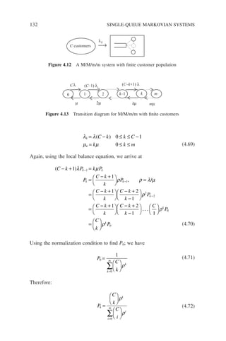
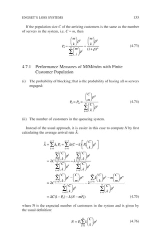
![134 SINGLE-QUEUE MARKOVIAN SYSTEMS
But we know that
N T
= = ×
λ λ
µ
1
therefore
N C P N mP
N C C m P
b b
b
= − − −
=
+
−
+
−
1
1
1 1
µ
λ λ
ρ
ρ
ρ
ρ
[ ( ) ( )]
( ) (4.77)
where
ρ
λ
µ
=
If the population size C of the arriving customers is the same as the number
of servers in the system, i.e. C = m, then
N m
=
+
ρ
ρ
1
(4.78)
(iii) The system time
T =
1
µ
(4.79)
4.8 CONSIDERATIONS FOR APPLICATIONS OF
QUEUEING MODELS
Those queueing models discussed so far are fairly elegant in analysis and yield
simple closed-form results owing to the memoryless property of Poisson
process and exponential service times. However, how valid are the assump-
tions of Poisson arrival process and exponential service times in real-life
applications?
From the past observation and studies, the Poisson arrival has been found
to be fairly accurate in modelling the arrival of calls in a telephone network,
and hence was extensively used in designing such networks. It is a fairly good
model as long as the arriving customer population is large and there is no
interdependency among them on arrival. It may not fully match the arrival](https://image.slidesharecdn.com/qtts-230925120453-047b3b23/85/QTTS-pdf-157-320.jpg)

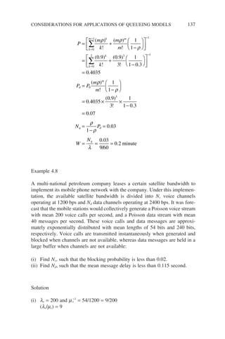
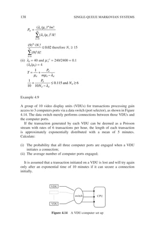
![Solution
In this example, computer ports are servers and transactions are customers and
the problem can be formulated as an M/M/m/m system with finite arriving
customers.
Given l = 6/60 = 0.1 trans/min m−1
= 5 min therefore a = 0.5
(i)
P
k
b
k
k
=
=
=
∑
10
3
0 5
10
0 5
0 4651
3
0
3
( . )
( . )
.
(ii) N =
+
× −
+
− ×
=
0 5
1 0 5
10
0 5
1 0 5
10 3 0 4651
2 248
.
.
.
.
( ) .
.
Problems
1. By referring to Section 4.1, show that the variance of N and W for
an M/M/1 queue are
(i) Var[N] = r/(1 − r)2
(ii) Var[W] = [m(1 − r)]−2
2. Show that the average number of customers in the M/M/1/S model
is N/2 when l = m.
3. Consider an M/M/S/S queueing system where customers arrive from
a fixed population base of S. This system can be modelled as a
Markov chain with the following parameters:
λ λ
µ µ
k
k
s k
k
= −
=
( )
Draw the state-transition diagram and show that the probability of an
empty system is (1 + r)−S
. Hence find the expected number of cus-
tomers in the system.
4. Data packets arrive at a switching node, which has only a single
output channel, according to a Poisson process with rate l. To
handle congestion issues, the switching node implements a simple
strategy of dropping incoming packets with a probability p when
the total number of packets in the switch (including the one
under transmission) is greater or more than N. Assuming that the
CONSIDERATIONS FOR APPLICATIONS OF QUEUEING MODELS 139](https://image.slidesharecdn.com/qtts-230925120453-047b3b23/85/QTTS-pdf-162-320.jpg)

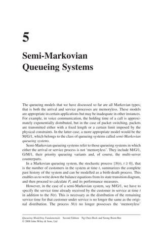
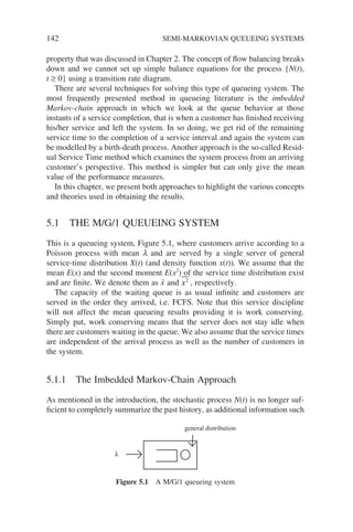
![THE M/G/1 QUEUEING SYSTEM 143
as the elapsed service time x0(t) needs to be specified. If we also specify the
elapsed service time, then the tuple [N(t), x0(t)] is again a Markov process and
we will be able to proceed with the analysis using Markov theory. Unfortu-
nately, this is a two-dimensional specification of the state space and compli-
cates the analysis considerably.
However, we can simplify the [N(t), x0(t)] specification into a one-
dimensional description N(t) by selecting certain special observation instants
in time. If we observe the M/G/1 queue at departure instants {rn}, where
x0(t) = 0, then we have a one-dimensional state space specification. The evolu-
tion of the number of customers N(t) left behind by a departing customer at
these instants is an imbedded Markov chain and we can again resort to Markov
theory to derive the desired performance measures.
But before we proceed, let us take a closer look at the state description N(t)
at those departure epochs. This is the state probability that is seen by a depart-
ing customer. Is it the same as the limiting steady-state probability which is
the system state observed by a random observer?
Fortunately, it can be shown that the system state seen by a departing cus-
tomer is the same as the system state seen by an arriving customer. Kleinrock
(1975) reasoned that the system state in an M/G/1 queue can change at most
by +1 or −1. The former corresponds to a customer arrival and the latter refers
to a departure. In the long term, the number of transitions upwards must equal
the number of transitions downwards. Hence the system state distribution seen
by a departing customer should be the same as that seen by an arriving
customer.
And according to the PASTA property, as shown in Section 4.2, the system
state distribution seen by an arriving customer is the same as the limiting
steady-state distribution. We can therefore conclude that the system state dis-
tribution that we are going to derive with respect to a departing customer is
the same as the limiting steady-state distribution seen by a random observer,
that is the usual limiting state distribution we have been deriving for other
queues.
With the assurance that the imbedded Markov process will yield the same
limiting steady-state distribution, we can then proceed with our analysis.
5.1.2 Analysis of M/G/1 Queue Using Imbedded
Markov-Chain Approach
Let us focus our attention at the departure epochs and examine the number of
customers Nn left behind by customer Cn at the departure instant rn. If Cn left
behind a non-empty system, then customer Cn+1 will leave behind a system with
the number of customers increased by the number of arrivals during the service
time of customer Cn+1 minus themselves; that is Nn+1 = Nn − 1 + An+1, where
An+1 is the number of arrivals during the service time of customer Cn+1.](https://image.slidesharecdn.com/qtts-230925120453-047b3b23/85/QTTS-pdf-166-320.jpg)
![144 SEMI-MARKOVIAN QUEUEING SYSTEMS
However, if Cn leaves behind an empty queue, then the service does not start
until Cn+1 arrives. The number of customers left behind will merely be the
number of arrivals during his/her service time, that is Nn+1 = An+1. Combining
both scenarios, we have
N N A
n n n
+
+
+
= − +
1 1
1
( ) (5.1)
where we have used the notation (x)+
= max(x, 0). Note that An+1 only depends
upon the length of the service time (xn+1) of Cn+1 and not upon n at all, hence
we can drop the subscript n. If we denote the probability of k arrivals in the
service period of a typical customer as
a P A k
k = =
[ ] (5.2)
then on condition that x = t and using the law of total probability together with
the fact that A is Poisson distributed with parameter lt as the arrival process
of M/G/1 queue is Poisson, we have
a P A k P A k x t x t dt
t
k
e x t d t
k
k
t
= = = = =
=
∞
∞
−
∫
∫
[ ] [ | ] ( )
( )
!
( ) ( )
0
0
λ λ
(5.3)
By definition, the transition probabilities of this imbedded Markov chain are
given as
P P N j N i
ij n n
[ | ]
+ = =
1 (5.4)
Since these transitions are observed at departure instants, Nn+1 Nn − 1 is an
impossible event and Nn+1 ≥ Nn − 1 is possible for all values due to the arrivals
An+1, we have
P
a i j i
a i j
ij
j i
j
=
≥ −
= ≥
− +1 0 1
0 0
,
,
(5.5)
And the transition probability matrix P̃ = [Pij] is given as
P
a a a a
a a a a
a a a
a a a
=
0 1 2 3
0 1 2 3
0 1 2
0 1 2
0
0
(5.6)](https://image.slidesharecdn.com/qtts-230925120453-047b3b23/85/QTTS-pdf-167-320.jpg)
![THE M/G/1 QUEUEING SYSTEM 145
Given the service distribution, the transition probabilities are completely
defined by Equation (5.3) and theoretically the steady state distribution can be
found using p̃ = p̃P̃. Instead of pursuing this line of analysis, we derive the
system state using generating functions. We define the generating function of
A as
A z E z P A k z
A
k
k
( ) [ ] [ ]
= =
=
∞
∑
0
(5.7)
Using Equation (5.3), we have
A z
t
k
e x t dt z
e
tz
k
k
k
t k
t
k
k
( )
( )
!
( )
( )
!
= { }
=
=
∞
∞
−
∞
−
=
∞
∑ ∫
∫ ∑
0
0
0
0
λ
λ
λ
λ
=
= −
∞
− −
∫
x t dt
e x t dt
x z
z t
( )
( )
)
( )
0
λ λ
λ λ
*( (5.8)
where x*(l − lz) is the Laplace transform of the service time pdf, x(t), evalu-
ated at l − lz.
Expression (5.8) reveals an interesting relationship between the number of
arrivals occurring during a service interval x where the arrival process is
Poisson at a rate of l.
Let us evaluate the mean and second moment of A as we need them for the
subsequent analysis of system state. Using Equation (5.8), we have
A E A
dA z
dz
dx z
dz
dx z
d z
d z
d
z
z
[ ]
( )
)
( )
( )
( )
=
=
−
=
−
−
⋅
−
=
=
1
1
*(
*
λ λ
λ λ
λ λ
λ λ
z
z
dx z
d z
z
z
=
=
= − ⋅
−
−
1
1
λ
λ λ
λ λ
*( )
( )
(5.9)
But the last term is just the mean service time x̄, hence we arrive at
A x
= =
λ ρ (5.10)
Proceeding with the differentiation further, we can show that](https://image.slidesharecdn.com/qtts-230925120453-047b3b23/85/QTTS-pdf-168-320.jpg)
![146 SEMI-MARKOVIAN QUEUEING SYSTEMS
A E A
E x A
2 2
2 2
[ ]
[ ]
= +
λ (5.11)
5.1.3 Distribution of System State
Let us now return to our earlier investigation of the system state. We define
the z-transform of the random variable Nn as
N z E z P N k z
n
N
k
n
k
n
( ) [ ] [ ]
= =
=
∞
∑
0
(5.12)
Taking z-transform of Equation (5.1), we have
E z E z
N N A
n n
[ ] [ ]
( )
+
+
= − +
1 1
(5.13)
We drop the subscript of A as it does not depend on n. Note that A is also
independent of the random variable Nn, so we can rewrite the previous
expression as
E[zNn+1
] = E[z(Nn−1)
+
]E[zA
]
and combining the definition of their z-transform, we have
N z A z E Z
n
Nn
+
−
= ⋅
+
1
1
( ) ( ) [ ]
( )
(5.14)
Let us examine the second term on the right-hand side of the expression:
E z P N K z
P N P N K z
N
k
n
k
n
k
n
k
n
[ ] [ ]
[ ] [ ]
(
( ) ( )
−
=
∞
−
=
∞
−
+ +
= =
= = + =
=
∑
∑
1
0
1
1
1
0
1
1
1 1
0
1
1 1
0
− + = − =
= − + −
−
=
∞
∑
ρ
ρ
ρ
) [ ] [ ]
( ) ( )
z
P N K z
z
P N
z
N z
z
k
n
k
n
n (5.15)
We assume that the limiting steady-state exists, that is
N z N z N z
n
n
n
n
( ) ( ) ( )
= =
→∞ →∞
+
lim lim 1](https://image.slidesharecdn.com/qtts-230925120453-047b3b23/85/QTTS-pdf-169-320.jpg)
![THE M/G/1 QUEUEING SYSTEM 147
We then arrive at
N z
z A z
z A z
z x z
z x z
( ) ( )
( ) ( )
( )
( )
( ) ( )
( )
= −
−
−
= −
− −
− −
1
1
1
1
ρ
ρ
λ λ
λ λ
*
*
(5.16)
Having obtained the generating function of the system state given in Equation
(5.16), we can proceed to find the mean value N as
N E N t
d
dz
N z z
= = =
[ ( )] ( )| 1
With N we can proceed to calculate other performance measures of the M/G/1.
We will postpone this until we examine the Residual Service Time approach.
5.1.4 Distribution of System Time
System Time refers to the total time a typical customer spends in the system.
It includes the waiting time of that customer and its service time. Note that
though the distribution of system state derived in the previous sections does
not assume any specific service discipline, the system time distribution is
dependent on the order in which customers are served. Here, we assume that
the service discipline is FCFS. The Laplace transform of the system time dis-
tribution T(s) can be found using the extension of the concept adopted in the
previous section. We will briefly describe it as this is a commonly used approach
in analysing the delays of queueing systems.
Recall that in Section 5.1.2 we derived the generating function of the total
arrivals A during a service time interval x, where the arrival process is Poisson
with rate l given by A(z) = x*(l − lz). Similarly, since a typical customer
spends a system time T in the system, then the total arrivals during their system
time interval will be given by
A z
t
k
e f t dt z
T z
T
k
k
t
T
k
( )
( )
!
( )
)
= { }
= −
=
∞
∞
−
∑ ∫
0
0
λ
λ λ
λ
*( (5.17)
where AT(z) is the generating function of the total arrivals, fT(t) is the density
function of system time and T*(s) is the Laplace transform of the system
time.](https://image.slidesharecdn.com/qtts-230925120453-047b3b23/85/QTTS-pdf-170-320.jpg)
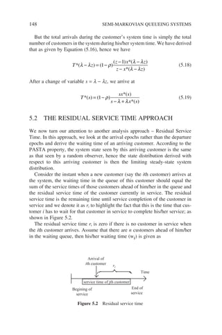
![w u k r x
i i
j i n
i
j
= +
= −
−
∑
( )
1
(5.20)
where u(k) is defined as follows to account for either an empty system or a
system with k customers:
u k
k
otherwise
( ) =
≥
{1 1
0
(5.21)
If the system is assumed to be ergodic and hence a steady-state exists, taking
expectation of both sides and noting that n is a random variable, we arrive at
E w E u k r E x
i i
j i n
i
j
[ ] [ ( ) ]
= +
= −
−
∑
1
(5.22)
Let us examine the first term on the right-hand side of the expression. Here
we assume that the service time distribution is independent of the state of the
system; that is the number of customers in the system. We have
E u k r E u k E r
P k P k E r
R xR
i i
i
[ ( ) ] [ ( )] [ ]
{ [ ] [ ]
} [ ]
=
= ⋅ = + ≥
= =
0 0 1
ρ λ
(5.23)
where R = E[ri] is the mean residual service time. The second term in Equation
(5.22) is simply the random sum of independent random variables and follows
the result of Example 1.7. Combining both results and Little’s theorem, we
obtain the following expressions:
E w xR E n E x
W xR xN xR x W
W
xR
i j
q
[ ] [ ] [ ]
= +
= + + +
=
−
λ
λ λ λ
λ
ρ
1
(5.24)
where Nq is the expected number of customers in the waiting queue and
W = E[wi].
The only unknown in Equation (5.24) is R. We note that the function of ri
is a series of triangles with the height equal to the required service time when-
ever a new customer starts service, and the service time decreases at a unit rate
until the customer completes service, as depicted in Figure 5.3. Note that there
are no gaps between those triangles because we are looking at ri conditioned
on the fact that there is at least one customer in the system and this fact is taken
care of by the u(k) in the expression (5.20).
THE RESIDUAL SERVICE TIME APPROACH 149](https://image.slidesharecdn.com/qtts-230925120453-047b3b23/85/QTTS-pdf-172-320.jpg)
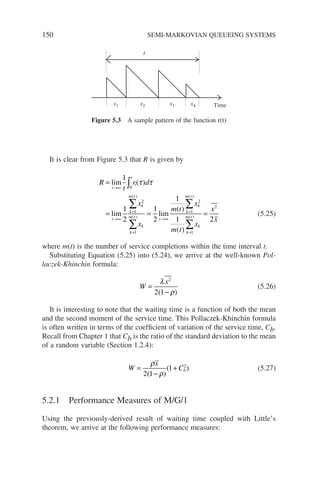
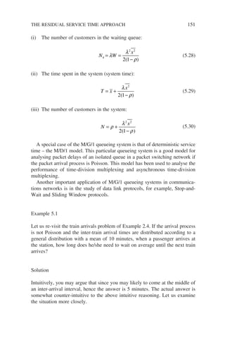
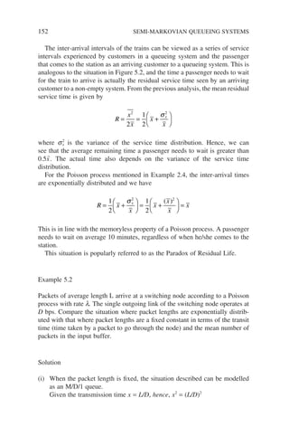
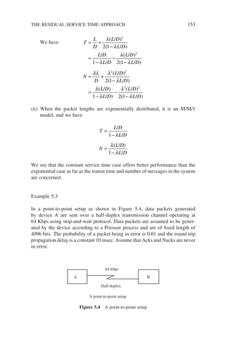
![154 SEMI-MARKOVIAN QUEUEING SYSTEMS
(i) What is the average time required to transmit a packet until it is correctly
received by B?
(ii) At what packet arrival rate will the transmission channel be saturated?
(iii) At half the arrival rate found in part (ii), what is the average waiting time
of a packet before it gets transmitted?
Solution
(i) From the data exchange sequence (Figure 5.5), it is clear that the probabil-
ity that it will take exactly k attempts to transmit a packet successfully is
pk−1
(1 − p), and
E n kp p
p
E n k p p p
k
k
k
k
k
[ ] ( )
[ ] ( ) ( )
= − =
−
= − = −
=
∞
−
=
∞
−
=
∞
∑
∑ ∑
1
1
2
1
2 1
1
1
1
1
1 1 k
k p
p
p p
p
p
k
2 1
3 2 2
1
2
1
1
1
1
1
−
= −
−
−
−
=
+
−
( )
( ) ( ) ( )
T transmission time round trip delay
L = +
= + =
( / ) . .
4096 64000 0 01 0 074s
s
and T E n TL
= ⋅ =
−
×
=
[ ]
.
.
.
1
1 0 01
0 074
0 07475s
(ii) Saturation occurs when the link utilization = 1, that is
λ µ
= = =
1
13 38
T
. packet/s
data ( p)
data (1–p)
data ( p)
Nack
Nack
Ack
TL
T
Figure 5.5 Data exchange sequence](https://image.slidesharecdn.com/qtts-230925120453-047b3b23/85/QTTS-pdf-177-320.jpg)
![(iii) The transmission channel can be modelled as an M/G/1 queue and the
waiting time in the queue is given by the Pollaczek-Khinchin formula.
Note that the rate now is 13.38/2 = 6.69.
E T T E n
W
E T
T
L
[ ] [ ] .
[ ]
( )
.
2 2 2 2
2
0 005643
2 1
0 0378
= ⋅ =
=
−
=
s
s
λ
λ
5.3 M/G/1 WITH SERVICE VOCATIONS
Parallel to those extensions we had for the M/M/1 queue, we can extend this
basic M/G/1 model to cater for some variation in service times. We shall look
at the case where the M/G/1 server takes a rest or so-called ‘vacation’ after
having served all the customers in the waiting queue. He/she may take another
vacation if the system is still empty upon his/her return. Customers arriving
during such vacation periods can go into service only after the server returns
from vacation. This model could be applied in a polling type situation where
a single server polls a number of stations in a pre-defined fashion. From the
station’s point of view, the server goes for a vacation after completing service
to all customers at this station.
Assume that those successive vacations taken by the server are independent
and identically distributed random variables. They are also independent of the
customer inter-arrival times and service times. Using the same reasoning as
before, the waiting time of a customer i in the queue before he/she receives
his/her service is given by
W u k r u k v x
i i i
j i n
i
j
= + ′ +
= −
−
∑
( ) ( )
1
(5.31)
where vi is the residual vacation time; that is the remaining time to completion
of a vacation when customer i arrives at the system, and u′(k) is the comple-
ment of the unit-step function defined in Equation (5.21). It is defined as
′ =
=
{
u k
u k
otherwise
( )
( )
0 1
1
We use this complement function to reflect the fact that when a customer arrives
at the system, he/she either sees a residual service time or falls into a vacation
period, but not both. From the previous section, we have
E[u(k)ri] = rRs
hence
M/G/1 WITH SERVICE VOCATIONS 155](https://image.slidesharecdn.com/qtts-230925120453-047b3b23/85/QTTS-pdf-178-320.jpg)
![156 SEMI-MARKOVIAN QUEUEING SYSTEMS
E[u′(k)vi] = (1 − r)Rv.
Here, we denote Rs as the mean residual service time and Rv as the mean
residual vacation time. As usual, taking expectation of Equation (5.31), we
have
W R R
s v
=
−
+
ρ
ρ
1
(5.32)
We already have the expression for Rs. To find Rv, we again examine the
function of residual vacation time, as shown in Figure 5.6. The busy periods
in between those vacation periods do not appear in the diagram because they
have been taken care of by the residual service time.
Following the same arguments as before, the mean residual vacation time
Rv is found to be
R
V
V
v =
1
2
2
(5.33)
Therefore, substituting into the expression for W, we obtain
W
x V
V
x
C
V
V
b
=
−
+
=
−
+ +
λ
ρ
ρ
ρ
2 2
2
2
2 1 2
2 1
1
2
( )
( )
( )
or
(5.34)
5.3.1 Performance Measures of M/G/1 with Service Vacations
(i) The system time:
T x
x V
V
= +
−
+
λ
ρ
2 2
2 1 2
( )
(5.35)
Time
v1 v2 v3 v4
t
Figure 5.6 A sample pattern of the function v(t)](https://image.slidesharecdn.com/qtts-230925120453-047b3b23/85/QTTS-pdf-179-320.jpg)
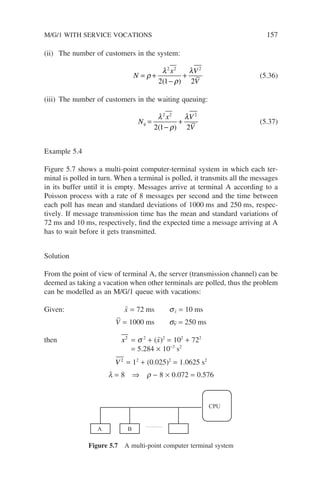
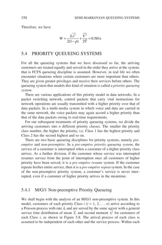
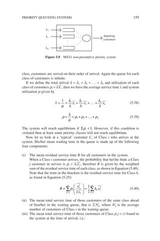
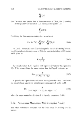
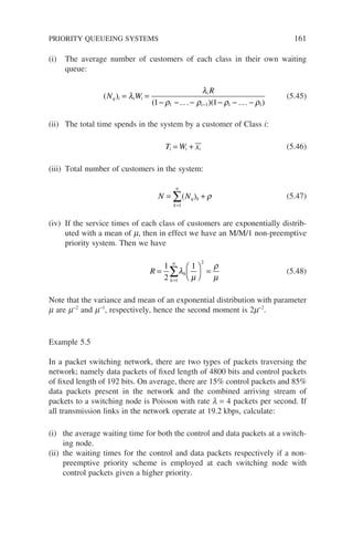
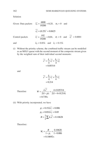
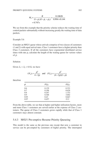
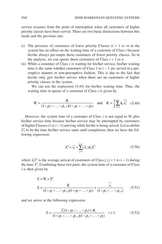
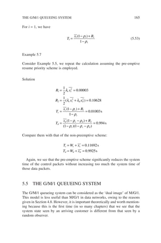
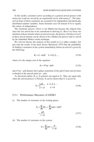
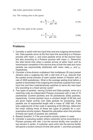
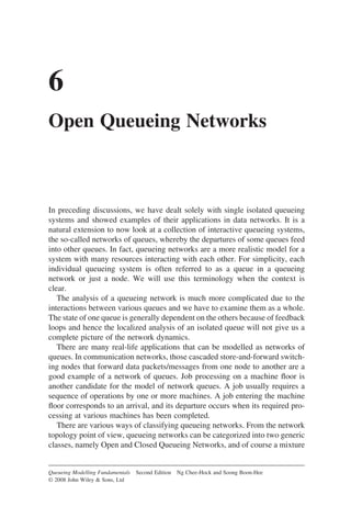
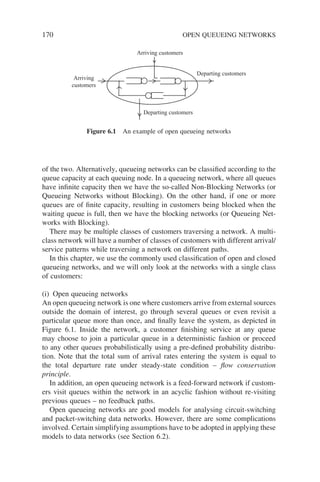
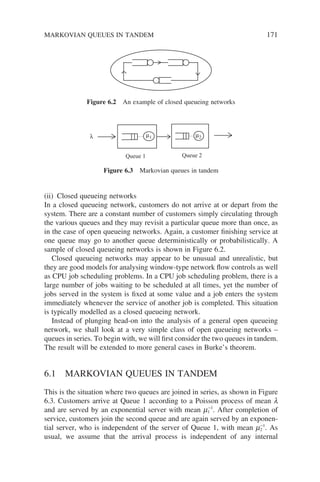
![172 OPEN QUEUEING NETWORKS
processes in both queues. The waiting time at both queues are assumed to be
infinite so that no blocking occurs. This is an example of a simple feedback
open network where no feedback path exists.
The analysis of this system follows the same approach as that of a single
Markovian queue except now we are dealing with a two-dimensional state space.
Let us focus our attention on the system state (k1, k2), where k1 and k2 are the
numbers of customers in Queue 1 and Queue 2, respectively. Since the arrival
process is Poisson and the service time distributions are exponential, we can have
only the following events occurring in an incremental time interval ∆t:
• an arrival at Queue 1 with probability l∆t;
• a departure from Queue 1, and hence an arrival at Queue 2, with probability
m1∆t;
• a departure from Queue 2 with probability m2∆t;
• no change in the system state with probability [1 − (l + m1 + m2)∆t].
Using the same technique that we employed in studying birth-death pro-
cesses, by considering the change in the joint probability P(k1, k2) in an infini-
tesimal period of time ∆t, we have
P k k t t P k k t t P k k t t
P k k
( , ; ) ( , ; ) ( , ; )
( ,
1 2 1 2 1 2 1
1 2
1 1 1
1
+ = − + + −
+ +
∆ ∆ ∆
λ µ
;
; ) ( , ; )[ ( ) ]
t t P k k t t
µ λ µ µ
2 1 2 1 2
1
∆ ∆
+ − + + (6.1)
Rearranging terms and dividing the equation by ∆t and letting ∆t go to zero,
we arrive at a differential equation for the joint probability:
′ = − + + −
+ + −
P k k t P k k t P k k t
P k k t
( , ; ) ( , ; ) ( , ; )
( , ; )
1 2 1 2 1 2 1
1 2 2
1 1 1
1
λ µ
µ P
P k k t
( , ; )[ ]
1 2 1 2
λ µ µ
+ + (6.2)
where P′(k1, k2; t) denotes the derivative. If l m1 and l m2, the tandem
queues will reach equilibrium. We can then obtain the steady-state solution by
setting the differentials to zero:
µ µ λ µ µ
λ
1 2 1 2 1 1 2 2 1 2
1 2
1 1 1
1
+ +
( ) = + − + +
+ −
P k k P k k P k k
P k k
( , ) ( , ) ( , )
( , ) (6.3)
Using the same arguments and repeating the process, we obtain three other
equations for the boundary conditions:
λ µ
P P
( , ) ( , )
0 0 0 1
2
= (6.4)
( ) ( , ) ( , ) ( , )
µ λ µ µ
2 2 1 2 2 2 2
0 1 1 0 1 0
+ = − + +
P k P k P k k (6.5)
( ) ( , ) ( , ) ( , )
µ λ µ λ
1 1 2 1 1 1
0 1 1 0 0
+ = + −
P k P k P k k (6.6)](https://image.slidesharecdn.com/qtts-230925120453-047b3b23/85/QTTS-pdf-195-320.jpg)
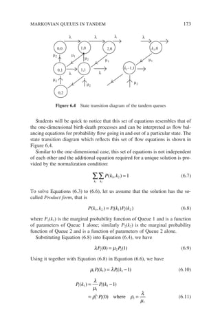
![174 OPEN QUEUEING NETWORKS
Since the marginal probability should sum to one, we have
P k P k
k k
1 1 2 2
1 2
1 1
∑ ∑
= =
( ) ( )
and (6.12)
Using the expression (6.12), we obtain P1(0) = (1 − r1), therefore
P k k
1 1 1 1
1 1
( ) ( )
= − ρ ρ (6.13)
Now, substituting Equations (6.10), (6.8) and (6.9) into Equation (6.3) and
after simplifying terms, we arrive at
( ) ( ) ( ) ( )
λ µ λ µ
+ = − + +
2 2 2 2 2 2 2 2
1 1
P k P k P k (6.14)
This is a recursive equation in P2(k2), which we solve by z-transform:
P k z P k z P k z
k
k
k
k
k
2 2
1
2 2
1
2 2
1
2 2
2
2
2
2
2
1 1
( )( ) ( ) ( )
=
∞
=
∞
=
∞
∑ ∑ ∑
+ = − + +
λ µ λ µ k
k2
(6.15)
Define the z-transform of P2(k2) as
P z P k z
k
k
2 2 2
0
2
2
( ) ( )
=
=
∞
∑ (6.16)
We have from Equation (6.15):
( )[ ( ) ( )] ( ) ( ) ( ) ( )
λ µ λ
µ λ
µ
+ − = + − −
P z P zP z
z
P z P P
P
2 2 2
2
2 2
2
2
2
0 0 0
(
( )( )( ) ( )( )( )
z z z P z
ρ ρ ρ λ µ
2 2 2 2 2
1 1 0 1 1
− − = + − =
where /
and
P z P
z
2 2
2
2
0
1
1
( ) ( )
=
+
−
ρ
ρ
(6.17)
Similarly, since the marginal probability P2 should sum to 1, that is equivalent
to P2(z)|z=1 = 1, we arrive at
P2
2
2
0
1
1
( ) =
−
+
ρ
ρ
(6.18)
and
P z
z
2 2
2
1
1
1
( ) ( )
= −
−
ρ
ρ
(6.19)](https://image.slidesharecdn.com/qtts-230925120453-047b3b23/85/QTTS-pdf-197-320.jpg)
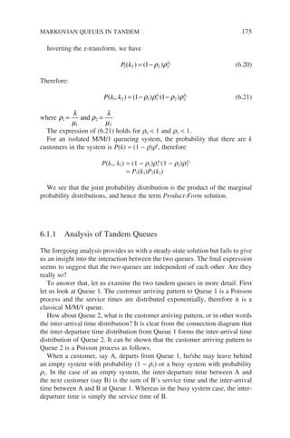
![176 OPEN QUEUEING NETWORKS
Therefore, the Laplace transform of the density function for the uncondi-
tional inter-departure time (I) between A and B is given by
L f t
s s s
s
I
[ ( )] ( )
= −
+
⋅
+
+
+
=
+
1 1
1
1
1
1
1
ρ
λ
λ
µ
µ
ρ
µ
µ
λ
λ
(6.22)
This is simply the Laplace transform of an exponential density function. Hence
a Poisson process driving an exponential server generates a Poisson departure
process. Queue 2 can be modelled as an M/M/1 queue.
6.1.2 Burke’s Theorem
The above discussion is the essence of Burke’s theorem. In fact, Burke’s
theorem provides a more general result for the departure process of an M/M/m
queue instead of just the M/M/1 queue discussed earlier. This theorem states
that the steady-state output of a stable M/M/m queue with input parameter l
and service-time parameter m for each of the m servers is in fact a Poisson
process at the same rate l. The output is independent of the other processes in
the system.
Burke’s theorem is very useful as it enables us to do a queue-by-queue
decomposition and analyse each queue separately when multiple-server queues
(each with exponential pdf service-times) are connected together in a feed
forward fashion without any feedback path.
Example 6.1
Sentosa Island is a famous tourist attraction in Singapore. During peak hours,
tourists arrive at the island at a mean rate of 35 per hour and can be approxi-
mated by a Poisson process. As tourists complete their sightseeing, they queue
up at the exit point to purchase tickets for one of the following modes of trans-
portation to return to the mainland; namely cable car, ferry and mini-bus. The
average service time at the ticket counters is 5 minutes per tourist.
Past records show that a tourist usually spends an average of 8 hours on
sightseeing. If we assume that the sightseeing times and ticket-purchasing
times are exponentially distributed; find:
i) the minimum number of ticket counters required in operation during peak
periods.](https://image.slidesharecdn.com/qtts-230925120453-047b3b23/85/QTTS-pdf-199-320.jpg)
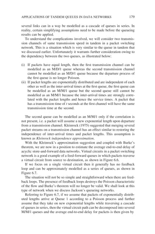
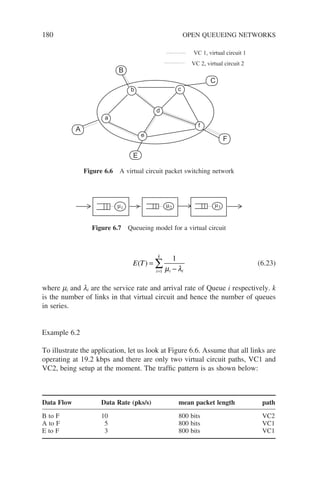
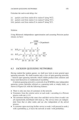
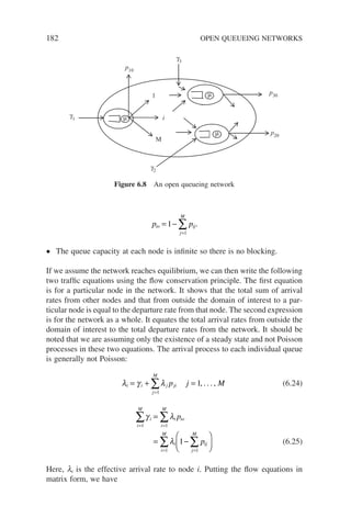
![λ λ γ
i j ji
j
M
i
p i M
− = =
=
∑
1
1 2
, , ... , (6.26)
I P
I P
T
T
λ λ γ
λ γ
− =
− =
( )
(6.27)
where
I
T
M
T
M
is the identity matrix
λ λ λ λ
γ γ γ γ
=
=
[ , , . . . , ]
[ , , . . . , ]
1 2
1 2
P
P
p p p
p p
p p
M
M MM
=
11 12 1
21 22
1
. . .
. . .
. . . . . . . . . . . .
(6.28)
Jackson demonstrated in 1957 (Jackson 1957) that the joint probability dis-
tribution for this type of network exhibits the product-form solution. i.e.:
P n P n n n
P n P n P n
M
M M
( ) ( , , ... , )
( ) ( ) ... ( )
=
=
1 2
1 1 2 2 (6.29)
where Pi(ni) is the marginal probability distribution of each node i.
We present here a simple verification of the product-form solution assuming
that all nodes are in an M/M/1 queue. In fact, the Jackson’s result is applicable
to multi-server and state dependent cases. To begin with, we define the follow-
ing notations:
ñ = (n1, n2, . . . , ni, . . . , nM)
1̃i = (0, 0, . . . , 1, 0, 0)
ñ − 1̃i = (n1, n2, . . . , ni − 1, . . . , nM)
ñ + 1̃i = (n1, n2, . . . , ni + 1, . . . , nM)
Parallel to the analysis of tandem queues, we again focus our attention on
the change in system state ñ in an incremental time interval ∆t. The system as
a whole is Markov because the arrival processes are all Poisson and service
processes are exponential, therefore there can only be four types of transition,
as follows:
JACKSON QUEUEING NETWORKS 183](https://image.slidesharecdn.com/qtts-230925120453-047b3b23/85/QTTS-pdf-206-320.jpg)
![184 OPEN QUEUEING NETWORKS
• no change in system state
• an arrival to node i
• a departure from node i
• transfer of a customer from node i to node j.
The corresponding transitional probability for the network going from state
m̃ to state ñ due to the above mentioned four events is
P n m
t t m n
t m n
p
i
i
M
i
i
M
i i
i ij
j
M
( )
=
− − =
= +
−
= =
=
∑ ∑
1
1
1
1 1
1
γ µ
γ
µ
∆ ∆
∆
∑
∑
= −
= + −
∆
∆
t m n
p t m n
i
i ij j i
1
1 1
µ
Therefore
P n t t P n t t t
P n t
i
i
M
i
i
M
[ ( )] [ ( )]
[ ( )
+ = − −
+ −
= =
∑ ∑
∆ ∆ ∆
1
1
1 1
γ µ
i
i i
i
M
i i ij
j
M
i
M
t P n t p t
P n t
] [ ( ) ]
[ ( )
γ µ
∆ ∆
= =
=
∑ ∑
∑
+ + −
+
1 1
1
1 1
+
+ −
=
=
∑
∑
1 1
1
1
j i j ji
j
M
i
M
p t
]µ ∆ (6.30)
Rearranging terms, dividing the equation by ∆t, taking limit and dropping the
time parameter, we have
d
dt
P n P n P n
P n
i
i
M
i
i
M
i i
i
M
( ) ( ) ( )
(
= − −
+ −
+
= = =
∑ ∑ ∑
γ µ γ
1 1 1
1
+
+ −
+ + −
=
= =
=
∑
∑ ∑
∑
1 1 1 1
1
1 1
1
i i ij
j
M
i
M
j ji
j
M
i
M
j i
p p P n
) ( )
µ µ (6.31)
Setting the derivative of the joint probability density function to zero, we
obtain
γ µ γ µ
i
i
M
i
i
M
i i
i
M
i ij
j
M
P n P n p
= = = =
∑ ∑ ∑ ∑
+
= − + −
1 1 1 1
1 1
( ) ( )
+
+ − +
=
=
=
∑
∑
∑
P n
p P n
i
i
M
j ji i j
j
M
i
M
( )
( )
1
1 1
1
1
1
µ (6.32)](https://image.slidesharecdn.com/qtts-230925120453-047b3b23/85/QTTS-pdf-207-320.jpg)
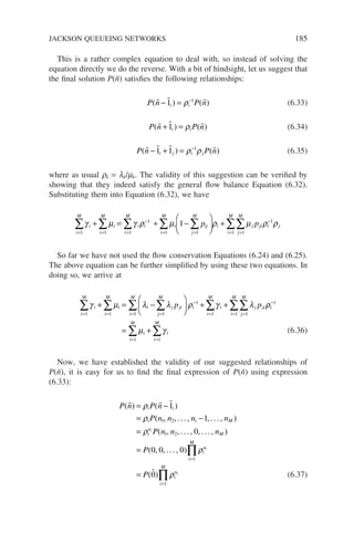
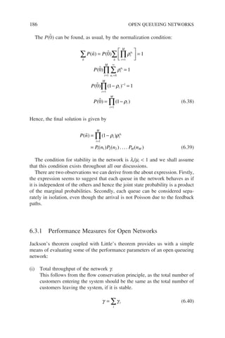
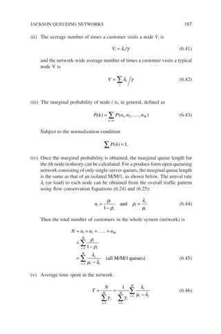
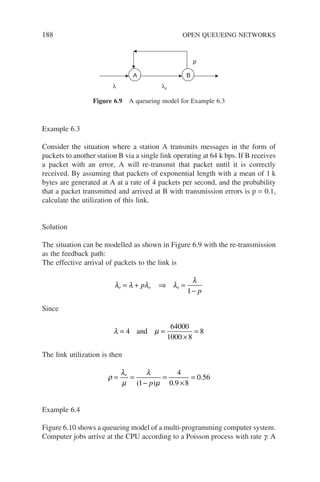
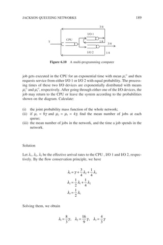
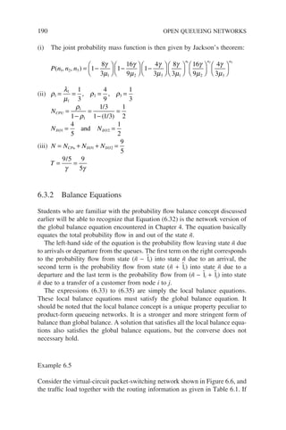
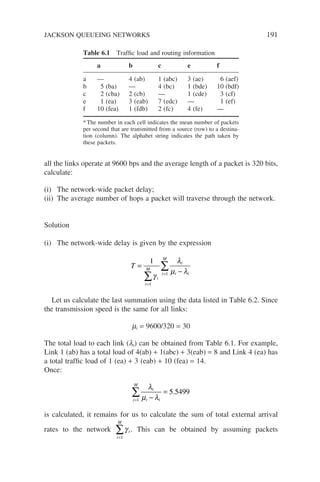
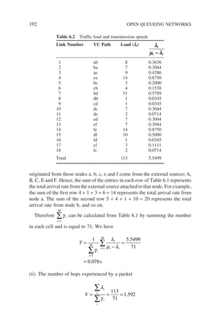
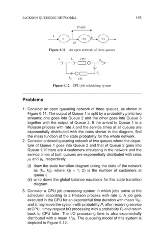
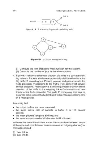
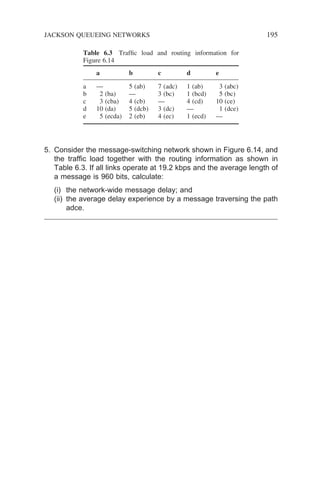

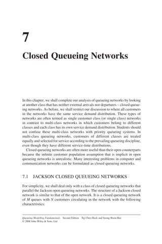
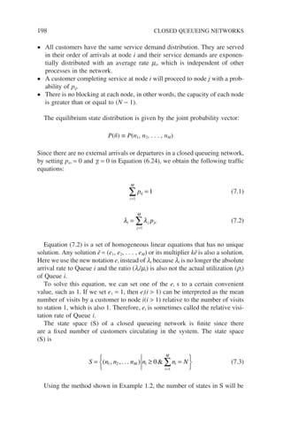
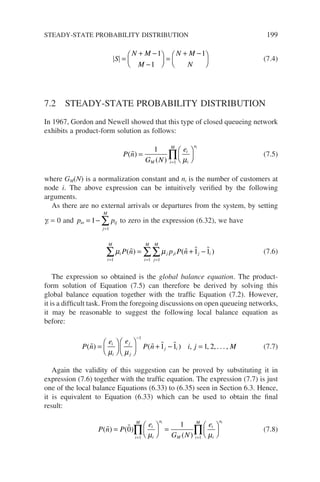
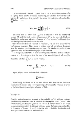
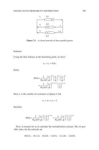
![202 CLOSED QUEUEING NETWORKS
Hence
G N
e e
M
i
i
n
i
M i
( ) =
=
+
+
=
∏ µ µ
1
1
2 2 2
1
2
1
2
1
2
+ + +
=
⊂
∑
2
1
2
1
2
1
2
1
11
4
n S
e
µ
Therefore, we have
P n
n
( )
=
−
4
11
1
2
2 1
The utilization of Queue 1 can be calculated as follows. Firstly, let us cal-
culate the probability that Queue 1 is idle:
P Q is idle P P P
[ ] ( , , ) ( , , ) ( , , )
1 0 0 2 0 1 1 0 2 0
3
11
= + +
=
Hence, the utilization of Queue 1 = 1 1
8
11
− =
P Q is idle
[ ]
Example 7.2
Again consider the closed queueing network shown in Figure 7.1. Let us inves-
tigate the underlying Markov chain for this queueing network. For the six
possible states (n1, n2, n3) mentioned in the previous example, the state transi-
tion diagram is shown in Figure 7.2.
µ(1–p)
µ(1–p)
µp
µp
µp
µ
µ
µ
µ
µ
µ
µ(1–p)
002
101 011
110
200 020
Figure 7.2 Transition diagram for Example 7.2](https://image.slidesharecdn.com/qtts-230925120453-047b3b23/85/QTTS-pdf-225-320.jpg)
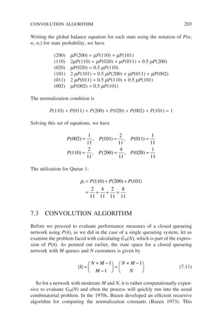
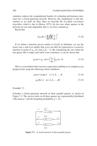
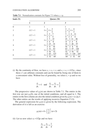
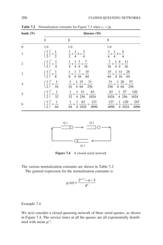
![In this case, we have e1 = e2 = e3. Let us fix the e1 = (1/2)m and we have
(ei/m) = 1/2. The progressive values of gm(n) are shown in Table 7.3.
7.4 PERFORMANCE MEASURES
From our early discussions of single-queue systems, we know that once the
steady-state probability distribution is obtained we can calculate the queueing
parameters that are of interest to us. As pointed out earlier, this approach could
lead to computational problems for even moderately sized closed queueing
networks. Fortunately, a number of important performance measures can be
computed as functions of the various normalization constants GM(N), which
can be evaluated by the recursive convolution algorithm.
In this section, we summarize some performance measures of a closed
queueing network in terms of GM(N) for the case of state-independent
queues:
(i) The number of customers at Queue i (Marginal queue length)
By definition, the marginal distribution is
P n P N n P n i M
i i
n S
n n
i
( ) [ ] ( ) , , . . .
= = = =
∈
=
∑
1 2 (7.16)
Table 7.3 Normalization constants for Figure 7.4
loads (N) Queues (M)
1 2 3
0 1.0 1.0 1.0
1
1
2
1
2
1
=
1
2
1
2
1
2
2
+ ⋅ =
2
2
1
2
1
3
2
+ ⋅ =
2
1
2
1
4
2
=
1
4
1
2
2
2
3
14
+ ⋅ =
3
4
1
2
3
2
6
4
+ ⋅ =
3
1
2
1
8
3
=
1
8
1
2
3
4
4
8
+ ⋅ =
4
8
1
2
6
4
10
8
+ ⋅ =
4
1
2
1
16
4
=
1
16
1
2
4
8
5
16
+ ⋅ =
5
16
1
2
10
8
15
16
+ ⋅ =
5
1
2
1
32
5
=
1
32
1
2
51
16
6
32
+ ⋅ =
9
32
1
2
15
16
21
32
+ ⋅ =
6
1
2
1
64
6
=
1
64
1
2
6
32
7
64
+ ⋅ =
7
64
1
2
21
32
28
64
+ ⋅ =
PERFORMANCE MEASURES 207](https://image.slidesharecdn.com/qtts-230925120453-047b3b23/85/QTTS-pdf-230-320.jpg)
![208 CLOSED QUEUEING NETWORKS
From Chapter 1 Equation (1.8), we see that Pi(n) can also be computed as
P n P N n P N n
i i i
( ) [ ] [ ]
= ≥ − ≥ +1 (7.17)
However
P N n P n
g N
e
i
n S
n n
M
j
j
n
j
M
n S
n n
i
j
i
[ ] ( )
( )
≥ = =
∈
≥
=
∈
≥
∑ ∏
∑
1
1 µ
(7.18)
Since Queue i has more than n customers, we can factor out (ei/mi)n
from the
last product term, and what remains is simply the normalization constant with
N − n customers. Hence
P N n
e g N n
g N
i
i
i
n
M
M
[ ]
( )
( )
≥ =
−
µ
(7.19)
Substituting back into Equation (7.17), we have
P n
e
g N
g N n
e
g N n
i
i
i
n
M
M
i
i
M
( )
( )
( ) ( )
=
− −
− −
µ µ
1
1 (7.20)
(ii) The mean number of customers at Queue i
The mean number of customers at Queue i is by definition
E N kP N k
i i
k
N
[ ] [ ]
= =
=
∑
1
(7.21)
But from Example 1.8 in Chapter 1, we know that the expected value of a dis-
crete random variable can alternatively be computed as
E N P N k
e g N k
g N
i i
k
N
i
i
k
M
M
k
N
[ ] [ ]
( )
( )
= ≥
=
−
=
=
∑
∑
1
1 µ
(7.22)
(iii) Marginal utilization of node i
For a single-server queueing network, the marginal utilization of node i is
ρ
µ
i i i
i
i
M
M
P N P N
e g N
g N
= − = = ≥
=
−
1 0 1
1
[ ] [ ]
( )
( )
(7.23)](https://image.slidesharecdn.com/qtts-230925120453-047b3b23/85/QTTS-pdf-231-320.jpg)
![(iv) Marginal throughput of node i
For a single-server and state-independent network, the throughput is by
definition
Ψi i i
k
N
i i
i
i
i
M
M
N P N k
P N
e g N
g N
( ) [ ]
[ ]
( )
( )
= =
= ≥
=
−
=
∑µ
µ
µ
µ
1
1
1
=
−
e
g N
g N
i
M
M
( )
( )
1
(7.24)
(v) The mean waiting time at Queue i
T
E N
e g N k
e g N
i
i
i
i i
k
M
k
N
i M
= =
−
−
=
∑
( )
( / ) ( )
( )
Ψ
µ
1
1
(7.25)
Example 7.5
Let us now calculate some performance measures of Queue 1 for the network
shown in Example 7.3:
(i) For the case of e1 1 1
µ = and e e
2 2 3 3 1 2
µ µ
= = , let us assume that
N = 5. We have from Section 7.4:
P N
e
g N
g N n
e
g N n
i
i
n
M
M
i
i
M
[ ]
( )
( ) ( )
1 2
1
1
= =
− −
− −
µ µ
=
= −
=
( ) ( )
1
32
120
26
8
1
11
4
2
15
2
E N
e g N k
g N
i
i
k
M
M
k
N
[ ]
( )
( )
1
1
32
120
57
16
26
8
11
4
4
2
1
=
−
= + + + +
=
∑ µ
=
67
20
Ψ1 5
57
16
32
120
19
20
( )
( )
( )
=
−
= ×
=
e
g N k
g N
i
M
M
µ µ
PERFORMANCE MEASURES 209](https://image.slidesharecdn.com/qtts-230925120453-047b3b23/85/QTTS-pdf-232-320.jpg)
![210 CLOSED QUEUEING NETWORKS
(ii) In the case of e1 1 1 2
µ = and e e
2 2 3 3 1 4
µ µ
= = and N = 5:
P N
[ ]
1
2
2
1
2
1024
120
26
64
1
2
11
16
2
15
= =
−
×
=
E N
( )
1
2 3 4
1024
120
1
2
57
256
1
2
26
64
1
2
11
16
1
2
4
4
=
+
+
+
+
+
=
1
2
1
67
20
5
Ψ1 5
57
256
1024
120
19
20
( ) = ×
=
µ µ
7.5 MEAN VALUE ANALYSIS
From the preceding examples, we see that substantial computation is involved
in evaluating the performance measures of a closed queueing network. Though
the convolution algorithm is meant to be implemented as a computer pro-
gram, the rapidly growing values of the progressive gm(n) can cause overflow/
underflow problems in the computing process.
In this section we present another technique called Mean Value Analysis
(MVA), which tackles the performance issue without the explicit evaluation of
normalization constants. This technique is due to Reiser and Lavenberg (Reiser
and Lavenberg 1980; Reiser 1982).
For simplicity, we shall look at the case where the service rates mi are state
independent. Again, focusing on the time a customer spends at a particular
queue, say the ith queue, we see that his/her queueing time is equal to his/her
service time plus that of those customers ahead of him/her. That is
Ti i i
= + ×
− −
µ µ
1 1
( )
average number of customers upon arrival (7.26)
Note that the residual service time of the customer in service does not
come into the equation because of the exponential service times. It has been
shown (Lavenberg and Reiser 1980) that for a closed queueing network that
has a product form solution, the number of customers in the queue seen by an
arriving customer at node i has the same distribution as that seen by a random
outside observer with one customer less. Therefore, the preceding equation can
be written as
T n N n
i i i
( ) [ ( )]
= + −
−
µ 1
1 1 (7.27)](https://image.slidesharecdn.com/qtts-230925120453-047b3b23/85/QTTS-pdf-233-320.jpg)
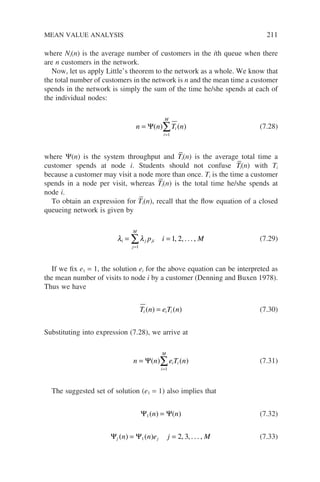
![212 CLOSED QUEUEING NETWORKS
Collecting Equations (7.27), (7.32) and (7.33), we have the set of recursive
algorithms for the network:
Ni(0) = 0 i = 1,2,3, . . . , M
Ti(n) = mi
−1
[1 + Ni(n − 1)
Ψ1
1
1
( ) ( )
n n e T n
i i
i
M
= ×
=
−
∑
Ψj = Ψi(n)ei j = 2,3, . . . M
Ni(n) = Ψi(n)Ti(n)
Example 7.6: Mean Value Analysis
We shall use Example 7.4 and calculate some of the performance parameters.
Since all the queues are connected in series, we have Ψi(n) = Ψ(n) and the set
of MVA algorithm reduced to
Ni(0) = 0 i = 1,2,3, . . . , M
Ti(n) = mi
−1
[1 + Ni(n − 1)]
Ψ( ) ( )
n n T n
i
i
M
= ×
=
−
∑
1
1
Ni(n) = Ψ(n)Ti(n)
We are given mi
−1
= m−1
, therefore we have
(i) First iteration, i.e. 1 customer in the network:
n̄i(0) = 0 i = 1,2,3
Ti(1) = m−1
[1 + n̄i(0)] = m−1
Ψ( ) ( )
1 1 1
3
1
3 1
= ×
=
=
−
∑Ti
i
µ
Ni(1) = Ψ(1) × m−1
= 1/3](https://image.slidesharecdn.com/qtts-230925120453-047b3b23/85/QTTS-pdf-235-320.jpg)
![(ii) Second iteration: i.e. 2 customers in the network:
Ti(2) = m−1
[1 + (1/3)] = 4/3 m
Ψ( ) ( )
2 2 2
2
1
3 1
= ×
=
=
−
∑Ti
i
µ
Ni(2) = Ψ(2) × (4/3 m) = 2/3
(iii) Third iteration: i.e. 3 customers in the network:
Ti(3) = m−1
[1 + (2/3)] = 5/3 m
Ψ( ) ( )
3 3 3
3
5
1
3 1
= ×
=
=
−
∑Ti
i
µ
Ni(3) = Ψ(3) × (5/3 m) = 1
7.6 APPLICATIONS OF CLOSED QUEUEING
NETWORKS
Closed queueing networks are well suited for modelling batch processing
computer systems with a fixed level of multi-programming. A computer system
can be modelled as a network of interconnected resources (CPU and I/O
devices) and a collection of customers (computer jobs), as shown in Figure 7.5.
This queueing model is known as the Central Server System in classical queue-
ing theory.
CPU
I/O M
I/O 1
p1
p2
p0
pM
Replacement loop
Figure 7.5 A central server queueing system
APPLICATIONS OF CLOSED QUEUEING NETWORKS 213](https://image.slidesharecdn.com/qtts-230925120453-047b3b23/85/QTTS-pdf-236-320.jpg)
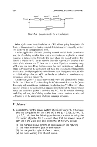
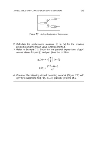

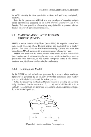
![The Markov-modulated Poisson process (MMPP) is a doubly stochastic
Poisson process whose rate varies according to a continuous time function. In
this case, the time function is the underlying Markov chain. MMPP is fully
characterized by the following parameters:
(i) The transition-rate matrix (also known as the infinitesimal generator
Q) of
the underlying modulating Markov process:
Q
q q q
q q q
q q
m
m
m m
=
−
−
−
1 12 1
21 2 2
1
(8.1)
where
q q
i ij
j
j i
m
=
=
≠
∑
1
We assume here that the transition-rate matrix
Q is homogeneous, i.e.
Q
does not vary with time. The steady-state vector:
π = [p1, p2, . . . , pm]
of the modulating Markov chain is then given by
π
Q = 0 and p1 + p2 + . . . + pm = 1
(ii) The Poisson arrival rate at each state l1, l2, . . . , lm. We define a diagonal
matrix
Λ and a vector
λ as
Λ =
=
diag m
m
( , , . . . )
λ λ λ
λ
λ
λ
1 2
1
2
0 0
0 0
0
0 0
(8.2)
λ λ λ λ
= ( , , . . . )
1 2 m
T
(8.3)
MARKOV-MODULATED POISSON PROCESS (MMPP) 219](https://image.slidesharecdn.com/qtts-230925120453-047b3b23/85/QTTS-pdf-242-320.jpg)
![220 MARKOV-MODULATED ARRIVAL PROCESS
(iii) The initial state (initial probability vector) of the MMPP, i.e.:
ϕ ϕ
i i
i
P J t i
= = = =
∑
[ ( ) ] .
0 1
Depending on the initial vector chosen, we have
(a) an interval-stationary MMPP that starts at an ‘arbitrary’ arrival epoch if the
initial vector is chosen as
ϕ
π λ π λ π λ
π
=
+ + +
1
1 1 2 2 . . . m m
Λ (8.4)
(b) an environment stationary MMPP whose initial probability vector is chosen
as
π, which is the stationary vector of
Q. Now the origin of time is not an
arrival epoch, but is chosen so that the environmental Markov process is
stationary.
Having described the model, let us examine the distribution of the inter-
arrival time of an MMPP. If we denote Xk as the time between (k − 1) arrival
and k arrival, and Jk the state of the underlying Markov process at the time of
the kth arrival, then the sequence {(Jk,Xk), k ≥ 0} is a Markov renewal sequence
with a transition probability distribution matrix given by
F x e d
e Q
I e
Q
x
Q x
( )
[ ( ) ]
{
[( ) ]
( )
(
=
= − −
= −
−
− −
∫ Λ
Λ
Λ
Λ Λ
ς
ς
ς
0
1
0
Q
Q x
Q
− −
−
Λ
Λ Λ
)
}( ) 1
(8.5)
The elements Fij(x) of the matrix are the conditional probabilities:
F x P J j X x J i
ij k k k
( ) { , }
= = ≤ =
−1 (8.6)
The transition probability density matrix is then given by differentiating
F(x) with respect to x:
f x
d
dx
F x e Q Q
e
Q x
Q x
( ) ( ) { ( )}( )
( )
( )
= = − − −
=
− − −
−
Λ
Λ
Λ Λ Λ
Λ
1
(8.7)
Taking the Laplace transform of
f (x), we have](https://image.slidesharecdn.com/qtts-230925120453-047b3b23/85/QTTS-pdf-243-320.jpg)
![L f x e e dx
sI Q e
Q x sx
sI Q
[ ( )]
[ ( )
( )
( )
=
= − − +
− −
∞
− − − +
∫ Λ
Λ
Λ
Λ
0
1 x
x
sI Q
]
( )
0
1
∞
−
= − +
Λ
Λ Λ (8.8)
Now let us consider N(t), the number of arrivals in (0, t). If J(t) is the state
of the Markov process at time t, define a matrix
P(n, t) whose (i, j) entry is
P n t P N t n J t j N t J t i
ij ( , ) [ ( ) , ( ) ( ) , ( ) ]
= = = = = = =
0 0 0 (8.9)
Then the matrices satisfy the Chapman–Kolmogorov equation and the matrix
generating function
P*(z, t) is
P z t P n t z
Q z t
n
n
*( , ) ( , )
exp{( ( ) ) }
=
= − −
=
∞
∑
0
1 Λ (8.10)
with
P z I
*( , )
0 = (8.11)
then the probability generating function of the number of arrivals is
g n t Q z t e
( , ) {exp( ( ) ) }
= − −
π 1 Λ (8.12)
where
π is the steady-state probability vector of the Markov chain and
e = [1, 1, . . . 1]T
.
Example 8.1
A two-state MMPP has only two states in its underlying modulating Markov
chain, characterized by
Q
r r
r r
=
−
−
=
1 1
2 2
1
2
0
0
and Λ
λ
λ
The stationary distribution is given by
π =
+ +
r
r r
r
r r
2
1 2
1
1 2
, .
MARKOV-MODULATED POISSON PROCESS (MMPP) 221](https://image.slidesharecdn.com/qtts-230925120453-047b3b23/85/QTTS-pdf-244-320.jpg)
![222 MARKOV-MODULATED ARRIVAL PROCESS
From Equation (8.8), we obtain
L f x
s
s
r r
r r
[ ( )]
=
−
−
−
+
{ }
−
0
0
0
0
0
0
1 1
2 2
1
2
1
1
λ
λ
λ
λ2
2
2 2 1
2 1 1
1
2
1 0
0
1
=
+ +
+ +
=
det
det
(
A
s r r
r s r
A
s
λ
λ
λ
λ
+
+ +
+ +
r r
r s r
2 2 1 2 1
1 2 1 1 2
λ λ λ
λ λ λ
)
( )
where
det A = (s + r1 + l1)(s + r2 + l2) − r1r2.
Without loss of generality, let us assume that this MMPP starts at an arrival
epoch. The stationary distribution of the Markov chain embedded at the arrival
instants is
ϕ
π
πλ λ λ
λ λ
= =
+
Λ 1
2 1 1 2
2 1 1 2
r r
r r
[ ]
Hence, the Laplace transform of the unconditional inter-arrival time is then
L X
A
s r r
r s r
[ ]
det
( )
( )
=
+ +
+ +
{ }
ϕ
λ λ λ
λ λ λ
1 1
1
2 2 1 2 1
1 2 1 1 2
=
=
+ + + + +
+
s r r r r r r
r r s
( ) ( )( )
( ){
1 2
2
2 1
2
1 2 2 1 1 2 1 2 2 1
1 2 2 1
2
λ λ λ λ λ λ λ λ
λ λ +
+ + + + + + +
( ) ( )}
r r s r r
1 2 1 2 1 2 1 2 2 1
λ λ λ λ λ λ
The interrupted Poisson process (IPP) is a special case of the two-state
MMPP, characterized by the following two matrices:
Q
r r
r r
IPP IPP
=
−
−
=
1 1
2 2
0
0 0
and Λ
λ
By setting l1 = l and l2 = 0 in the previous expression, we have the Laplace
transform of the inter-arrival times of an IPP as
L X
s r
s r r s r
s s
IPP
[ ]
( )
( )
( )
=
+
+ + + +
= −
+
+
+
2
2
1 2 2
1
1
2
2
1
λ
λ λ
β
α
α
β
α
α](https://image.slidesharecdn.com/qtts-230925120453-047b3b23/85/QTTS-pdf-245-320.jpg)
![where
α λ λ λ
1 1 2 1 2
2
2
1
2
4
= + + − + + −
( ) ( )
r r r r r
α λ λ λ
2 1 2 1 2
2
2
1
2
4
= + + + + + −
( ) ( )
r r r r r
β
λ α
α α
=
−
−
1
2 1
We note the expression for L[XIPP] is just the Laplace transform of a hyper-
exponential distribution with parameters (a1, a2) and branching probability
b. Therefore, the interrupted Poisson process is stochastically equivalent to a
hyper-exponential process.
8.1.2 Superposition of MMPPs
The superposition of n ≥ 2 independent Markov-modulated Poisson processes
with parameters
Q
Λi(i = 1,2, . . . , n) is again an MMPP with parameters
Q
Λ given by
Q Q Q Qn
= ⊕ ⊕ ⊕
1 2 . . . . . (8.13)
Λ Λ Λ Λ
= ⊕ ⊕ ⊕
1 2 . . . . . n (8.14)
where ⊕ denotes the Kronecter sum and is defined as
A B A I I B
B A
⊕ = ⊗ + ⊗
( ) ( ) (8.15)
and
C D
c D c D c D
c D c D c D
c D c D c D
m
m
n n nm
⊗ =
11 12 1
21 22 2
1 2
(8.16)
IA
I B are identity matrices with the same dimension as A and B, respec-
tively. Note that
Q
Λ are kxk matrices and k ni
i
n
=
=
∏
1
.
MARKOV-MODULATED POISSON PROCESS (MMPP) 223](https://image.slidesharecdn.com/qtts-230925120453-047b3b23/85/QTTS-pdf-246-320.jpg)
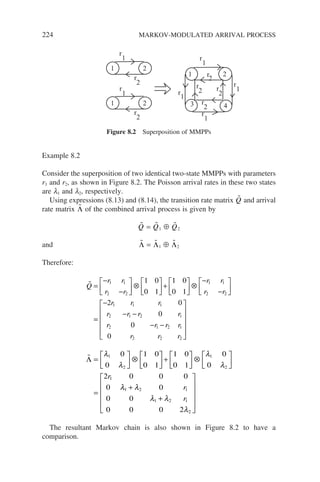
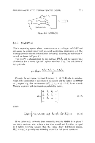
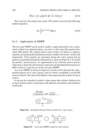
![8.2 MARKOV-MODULATED BERNOULLI PROCESS
The Markov-modulated Bernoulli Process (MMBP) is the discrete-time counter-
part of Markov-modulated Poisson Process (MMPP). Time in MMBPs is
discretized into fixed-length slots and the process spends a geometric duration
of time slots in each state. The probability that a slot containing an arrival is
a Bernoulli process, with a parameter that varies according to an m-state
Markov process, is independent of the arrival process.
8.2.1 Source Model and Definition
To serve as a teaching example, we consider only the two-state MMBP, as
shown in Figure 8.6, to simplify the analysis. In this model, the arrival process
has two distinct phases (or states); when the arrival process is in H-state in
time slot k, it generates an arrival with probability g and may remain in this
state in the next time slot (k + 1) with probability a. Similarly, when the arrival
process is in L-state in time slot k, it generates an arrival with probability z
and may remain in L-state in the next time slot (k + 1) with probability b. The
width of the time slots are taken to be the average service time in subsequent
analysis.
From the Markov theory, we know that the steady-state probability distribu-
tion
π = [pH, pL] for this two-state chain is given by
π
P =
π, where
P is the
state transition matrix:
P =
−
−
α α
β β
1
1 (8.21)
Solving the equation
π
P =
π together with pH + pL = 1, we have
π
β
α β
π
α
α β
H L
=
−
− −
=
−
− −
1
2
1
2
and (8.22)
H L
1-
1-
α β
α
β
Figure 8.6 A two-state MMBP
MARKOV-MODULATED BERNOULLI PROCESS 227](https://image.slidesharecdn.com/qtts-230925120453-047b3b23/85/QTTS-pdf-250-320.jpg)
![228 MARKOV-MODULATED ARRIVAL PROCESS
8.2.2 Superposition of N Identical MMBPs
Having presented the model of a single MMBP, we are now in a position to
examine the stochastic behaviour of superposing (multiplexing) a group of N
identical MMBPs. Firstly, let us define the following random variables:
a(k + 1) The number of traffic sources in H-state in slot (k + 1)
a(k) The number of traffic sources in H-state in slot k
b(k) The total number of cells generated by these N source in slot k
With a bit of thought, it can be shown that these random variables are related
as follows:
a k c d
j
j
a k
j
j
N a k
( )
( ) ( )
+ = +
= =
−
∑ ∑
1
1 1
(8.23)
b k s t
j
j
a k
j
j
N a k
( )
( ) ( )
= +
= =
−
∑ ∑
1 1
(8.24)
where cj, dj, sj and tj are random variables with the following definitions and
probability generating functions (PDFs):
c
with probability
with probability
F z
j H
=
−
{ = −
1
0 1
1
α
α
α
( )
( ) ( )
PDF is +
+αz
d
with probability
with probability
F z
j L
=
−
{ = + −
1 1
0
1
( )
( ) (
β
β
β
PDF is β
β)z
s
with probability
with probability
G z
j H
=
−
{ = −
1
0 1
1
γ
γ
γ
( )
( ) ( )
PDF is +
+ γ z
t
with probability
with probability
G z
j L
=
−
{ = −
1
0 1
1
ς
ς
ς
( )
( ) ( )
PDF is +
+ςz
Next, we define two matrices
A and
B whose (i, j) terms are
A i j P a k j a k i
( , ) [ ( ) ( ) ]
= + = =
1 (8.25)
B i j P b k j a k i
( , ) [ ( ) ( ) ]
= = = (8.26)](https://image.slidesharecdn.com/qtts-230925120453-047b3b23/85/QTTS-pdf-251-320.jpg)
![Matrix
A gives the correlation between the number of H-state MMBP sources
in adjacent time slots, and matrix
B shows the relationship between the number
of arrivals and the number of H-state MMBP sources in a particular time slot.
Both matrices are required in subsequent analysis.
To facilitate the build-up of these two matrices, we see that the z-transform
of the ith row of these two matrices are given respectively as
A z P a k j a k i z
F z F z
i
n
j
H
i
L
N i
( ) [ ( ) ( ) ]
( ) ( )
= + = =
= ⋅
=
∞
−
∑ 1
0
(8.27)
B z P b k j a k i z
G z G z
i
n
j
H
i
L
N i
( ) [ ( ) ( ) ]
( ) ( )
= = =
= ⋅
=
∞
−
∑
0
(8.28)
where f i
means the multiplication of i times.
The steady-state number of arrivals per time slot is then given by
λ π π
tot H H z L L z
N G z G z
= ′ + ′
= =
[ ( ) ( ) ]
1 1 (8.29)
8.2.3 ΣMMBP/D/1
In this section, we take a look at a queueing system where an infinite waiting
queue is fed by a group of N identical MMBP sources and served by a deter-
ministic server. Without loss of generality, we assume that the width of a time
slot is equal to the constant service time (1/m) and is equal to 1 unit of
measure.
Having obtained the correlation expressions (8.27) and (8.28) for those
random variables presented in the last section, we are now in a position to
examine the evolution of queue length in slot (k + 1), that is q(k + 1). Firstly, let
us define the z-transform of the joint probability P[q(k + 1) = j, a(k + 1) = i]:
Q z P q k j a k i z
z
i
k j
j
ji
k j
j
+
=
∞
+
=
∞
= + = + =
=
∑
∑
1
0
1
0
1 1
( ) [ ( ) , ( ) ]
π (8.30)
MARKOV-MODULATED BERNOULLI PROCESS 229](https://image.slidesharecdn.com/qtts-230925120453-047b3b23/85/QTTS-pdf-252-320.jpg)
![230 MARKOV-MODULATED ARRIVAL PROCESS
In matrix form, we have
Q z
Q z
Q z
z z
z
k
k
N
k
k o
j
k j
k o
j
+
+
+
+ +
+
=
=
1 0
1
1
00
1
0
1
01
1
( )
( )
( )
π π
π π 1
1
1
0
1 1
k j
N
k o
jN
k j
z
z z
+
+ +
π π
According to the model described, the queue will evolve according to
q k q k b k
( ) [ ( ) ] ( )
+ = − + +
+
1 1 1 (8.31)
where [a]+
denotes a or zero. If we examine Q0
k+1
(z) and expand it in terms of
those quantities in slot k using Equation (8.31), we will arrive at the following
expression after some lengthy algebraic manipulation:
Q z a B z
Q z
z
z
z
k
i
i
N
i
k
i
k
i
k
0
1
0 0
0
0 0
+
=
= +
−
∑
( ) ( )
( ) π π
(8.32)
where B0(z) is as defined in Equation (8.28). Similarly, we can derive similar
expressions for other terms Q1
k+1
(z), . . . , QN
k+1
(z). If we assume that
r = ltot/m
= N(pHG′
H(z)|z=1 + pLG′
L(z)|z=1)
1
then the queue system will reach an equilibrium and we have
lim ( ) lim ( ) lim ( )
k
k
k
k
k
Q z Q z Q z
→∞
+
→∞ →∞
= =
1
Putting all terms in matrix form, we have the following matrix equation:
Q z I
z
A
z
A
B
T
B
T
( ) = −
⋅ ⋅
−
1 1
1
Λ Λ Φ (8.33)
where
ΛB N
N
diag B z B z
B z
B z
B z
=
=
( ( ), . . . , ( ))
( )
( )
( )
0
0
1
0 0
0 0
(8.34)](https://image.slidesharecdn.com/qtts-230925120453-047b3b23/85/QTTS-pdf-253-320.jpg)
![Bi(z) is the z-transform defined in Equation (8.28) and
A is the matrix whose
rows are defined as in Equation (8.27) and
Φ =
−
−
−
π π
π π
π π
00 00
01 01
0 0
z
z
z
n N
(8.35)
Some interesting results can be observed from this expression. If we set
z = 1 in Equation (8.33), we have a set of linear equations as follows:
( ) ( )
zI A Q z A
a a
B
T
B
T
− ⋅ = ⋅
−
Λ Λ Φ
1 0 0
0 1
0
0 0 1
00 10
0 0
01 11 1
0 1
0
1
a
a a a
a a a
A
A
A
N
N
N N NN
⋅
N
N
=
0
0
0
Note that Ai is the steady-state probability of having i sources in H-state
and
Qi(z)|z=1 = Ai
= p0i + p1i + . . . + pNi
This is exactly the set of steady-state balance equations that governed the
behaviour of the set of N two-state Markov chains by solving the equation:
π
A =
π
8.2.4 Queue Length Solution
Earlier, we obtained an explicit expression (8.33) for the joint probability of
queue length and traffic source. However, we notice that the z-transform of
queue length (q) is given by
q z P q j z
Q z eQ z
j
j
i
i
N
( ) [ ]
( ) ( )
= =
= =
=
∞
=
∑
∑
0
0
(8.36)
MARKOV-MODULATED BERNOULLI PROCESS 231](https://image.slidesharecdn.com/qtts-230925120453-047b3b23/85/QTTS-pdf-254-320.jpg)
![232 MARKOV-MODULATED ARRIVAL PROCESS
From Equation (8.33) we have
Q z I
z
A
z
A
z A z
B
T
B
T
j
B
T j
j
( )
( )
= −
⋅ ⋅
=
−
− + −
=
1 1
1
1 1
0
Λ Λ Φ
Λ Φ
∞
∞
− − +
=
∞
∑
∑
= z A
j
B
T j
j
1 1
0
( )
Λ Φ (8.37)
From the section ‘Matrix Operation’ in Chapter 1, we know that
ΛB
AT
can
be expressed in terms of three matrices as
Λ Λ
B
T
i i i
i
N
A H z z H z
g h
=
=
−
=
∑
( ) ( ) ( )
1
0
λ (8.38)
where
H(z) is the eigenvector matrix of
ΛB
AT
and
Λ is a diagonal matrix con-
sisting of the corresponding eigenvalues of
ΛB
AT
.
gi is the column vector for
H(z) and
hi the row vector for
H−1
(z).
Substituting into Equation (8.37), we have
Q z z H z z H
z g h
j j
j
j
i
j
h i
i
N
( ) ( ( ) ( ) )
=
=
− − − +
=
∞
− − +
=
∑ 1 1 1
0
1 1
0
Λ Φ
λ
∑
∑
∑
∑
=
−
=
∞
=
∞
Φ
Φ
j
i
i
i i
j z
g h
0
0
λ
λ
(8.39)
To find the average queue length, let us take the derivative of
e
Q(z) when
z = 1:
E q eQ z
e I A A
z
T T
[ ] ( )
( )
= ′
= − ′
=
−
1
1
Φ (8.40)
where
Φ′ = (p00, . . . , p0N)T
.](https://image.slidesharecdn.com/qtts-230925120453-047b3b23/85/QTTS-pdf-255-320.jpg)
![8.2.5 Initial Conditions
To obtain queue length distribution, a group of initial conditions (initial condi-
tion vector Φ′) must first be determined. We define the system characteristic
function as Πi[z − li(z)] = 0. The roots of each equation (for each li) must be
one or more of the following three types:
(1) Vanishing roots : real roots and |z| ≤ 1,
(2) Non-vanishing roots : real roots and |z| 1,
(3) Ignored roots :complex roots.
Since
Q(z)must be finite in |z| ≤ 1, only vanishing roots are used for obtaining
initial conditions. For every vanishing root and for each given i, we can get an
initial condition equation
hi(z)Φ′ = 0. Since the Markov chain we discussed is
irreducible, it must have a root equal to 1, that is l0(1) = 1 must be true. For
this root, the initial condition equation is obtained by taking the limit of
e
Q(z)
in Equation (8.37) as z goes to 1, leading to
eg h
0 0 0
1 1 1 1
( ) ( )
′ = − ′ = −
Φ λ ρ (8.41)
This equation is used to solve the initial condition vector Φ′.
8.3 MARKOV-MODULATED FLUID FLOW
Fluid-flow modelling refers to continuous-space queues with continuous inter-
arrival times. In this type of modelling, we no longer treat the arrivals and depar-
tures as discrete units. The arrival process is deemed as a source of fluid flow
generating a continuous stream of arrivals that is characterized by a flow rate,
and departure as a continuous depletion of the waiting queue of a constant rate.
Fluid-flow models are appropriate approximations to situations where the
number of arrivals is relatively large so that an individual unit is by itself of
little significance. The effect is that an individual unit has only an infinitesimal
effect on the flow – like a droplet of water in a flow.
To adopt this model, the arrival traffic has to be heavy (r 90%) and hence
the waiting times in a queue are sufficiently large compared to the service time.
In this section, the arrival process is governed by a continuous-time Markov
process, and hence the term Markov-modulated fluid flow.
8.3.1 Model and Queue Length Analysis
As a teaching example, we consider a queueing system whose continuous
fluid arrival process is governed by a three-state Markov chain, as shown in
Figure 8.7.
MARKOV-MODULATED FLUID FLOW 233](https://image.slidesharecdn.com/qtts-230925120453-047b3b23/85/QTTS-pdf-256-320.jpg)
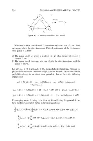
![Since we are interested in the steady-state behaviour of a queueing system, we
set
∂
∂
=
t
q t x
i ( , ) 0
hence we can drop the time parameter t and we have
( ) ( , ) ( ) ( , ) ( , ) ( , )
λ µ
− = − + + +
d
dx
q t x r r q t x r q t x r q t x
0 01 02 0 10 1 20 2 (8.42)
−
∂
∂
= − + +
µ
x
q t x r q t x r r q t x r q t x
1 01 0 10 12 1 21 2
( , ) ( , ) ( ) ( , ) ( , ) (8.43)
−
∂
∂
= + − +
µ
x
q t x r q t x r q t x r r q t x
2 02 0 12 1 21 20 2
( , ) ( , ) ( , ) ( ) ( , ) (8.44)
The qi(x) is the steady-state probability that the arrival process is in state i
and the queue length does not exceed x. In matrix form, we have
D
d
dx
Q x MQ x
( ) ( )
= (8.45)
where
Q x q x q x q x T
( ) ( ( ), ( ), ( ))
= 0 1 2
D diag
= − − −
[( ), , ]
λ µ µ µ
M
r r r r
r r r r
r r r r
=
− +
− +
− +
( )
( )
( )
01 02 10 20
01 10 12 21
02 12 21 20
From the section ‘Matrix Calculus’ in Chapter 1, we see that the general
solution of Equation (8.45) is
Q x Q a g e
i i
z x
i
( ) ( )
= ∞ + ∑ (8.46)
where the z′
is are eigenvalues of
D−1
M in the left-half complex plane (i.e.
Re(zi) 0) and gi are eigenvectors satisfying
zigi =
D−1
M
MARKOV-MODULATED FLUID FLOW 235](https://image.slidesharecdn.com/qtts-230925120453-047b3b23/85/QTTS-pdf-258-320.jpg)
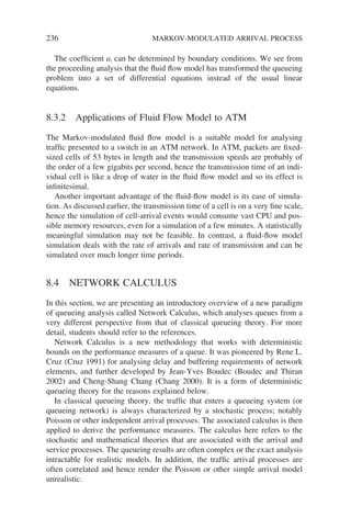
![However, in Network Calculus, the arrival traffic is assumed to be ‘unknown’
but only satisfies certain regularity constraints, such as that the amount of work
brought along by the arriving customers within a time interval is less than a
value that depends on the length of that interval. The associated calculus is
then developed to derive the deterministic bounds on the performance guaran-
tees. Hence, Network Calculus is also referred to as deterministic queueing.
The main difference between these two approaches – classical queueing
theory and Network Calculus – is that the former permits us to make statistical
predictions of performance measures whereas the later establishes determinis-
tic bounds on performance guarantees. For example, classical queueing theory
may predict that 90% of the time a customer would wait less than T seconds
before they receive their service, whereas the network calculus can ascertain
that the time taken to go through a queue is less than Y.
8.4.1 System Description
The main idea of the Network Calculus is analogous to that of the classical
system theory that has been long applied to electrical circuits. Given the input
function of a signal in classical system theory, the output can be derived from
the convolution of the input function and the impulse response function of the
system.
Similarly, we can consider a queueing system (or queueing network) as a
system. If we are able to put a constraint curve on the arrival process, then we
should be able to establish certain bounds on the output process by applying
certain calculus to both the arrival constraint curve and the ‘characteristic func-
tion’ of the queueing system. Figure 8.8 shows the schematic system view of
a queueing system.
In contrast to the conventional approach of characterizing the arrival proba-
bilistically using a stochastic process that counts the number of arrivals, we
focus our attention on the cumulative amount of work brought along to the
queueing system by customers. We describe the arrival process by a cumulative
function A(t), defined as the total amount of work brought to the queueing
system by customers in time interval [0, t]. Without loss of generality, we take
A(t) = 0 for t 0; in other word we assume that we begin with an empty system.
Arrival function
A(t)
Departure function
D(t)
Service function
b(t)
Figure 8.8 Schematic system view of a queue
NETWORK CALCULUS 237](https://image.slidesharecdn.com/qtts-230925120453-047b3b23/85/QTTS-pdf-260-320.jpg)
![238 MARKOV-MODULATED ARRIVAL PROCESS
Note that A(t) is the sum of the service times required by those arriving cus-
tomers in the time interval [0, t].
Similarly, instead of counting the number of departing customers from a
queueing system, we define an accumulative function D(t) as the total amount
of work completed by the queueing system in the time interval [0, t], in other
words, the completed services of those departed customers. Note that D(t) is
the cumulative amount of service time dispensed by the server in the time
interval [0, t], or the so-called finished work. Obviously:
D t A t D t for t
( ) ( ) ( )
≤ =
and 0 0 (8.47)
At the same time, we modify the usual description of system queue length.
The system queue length X(t) here refers to the total amount of service times,
so-called unfinished work, required by those customers in the system, rather
than the number of customers in the system.
Figure 8.9 shows a sample path of X(t) and its relationships to the arrivals.
A new arrival of a customer causes the X(t) to increase by the amount of work
brought along by this customer. If we assume that the server is serving custom-
ers at a constant rate C, then the waiting queue is depleted at rate C when it is
non-empty. The time periods during which the system content is non-empty
are called busy periods, and the periods during which the content is empty are
called idle periods.
It is obvious from Figure 8.9 that for a work-conserving system, the evolu-
tion of X(t) depends only on the arrival instants and the required service time
of that customer. Students should quickly realize that we have not made any
assumptions about the ways in which the customers arrive at the queue, nor
the service process. We only assume that the server dispenses his/her service
at a constant rate C.
Customer
c1 c2 c3 c4 c5
Time
Time
Amount
of
work
Figure 8.9 Arrivals and X(t) content](https://image.slidesharecdn.com/qtts-230925120453-047b3b23/85/QTTS-pdf-261-320.jpg)
![Assuming that the waiting queue is infinite, hence there is no overflow
during [0, t], the system queue length at time t is given by
X t A t A s X s C t s s t
( ) ( ) ( ) ( ) ( )
= − + − ⋅ −
0 (8.48)
A(t) − A(s) is the amount of work brought along by those customers in
[s, t], and C(t − s) is the amount of service that has been dispensed by the servers.
We assume here that A is left-continuous. To cater for the situation where there
is an arrival at t = 0 as well as the situation where the work arrival over [0, t]
had a rate less than C so that the queue never built up and X(t) = 0, we have
X t A t A s C t s
s t
( ) sup{ ( ) ( ) ( )}
= − − ⋅ −
≤
(8.49)
The short-hand notation ‘sup’ refers to ‘supremum’, which we will explain
in a later section. Similarly, we can derive an expression for the departure
process:
D t A t X t
A t A t A s C t s
A
s t
s t
( ) ( ) ( )
( ) sup{ ( ) ( ) ( )}
inf { (
= −
= − − − ⋅ −
=
≤
≤ ≤
−
0
s
s C t s
) ( )}
+ ⋅ − (8.50)
where ‘inf’ refers to ‘infimum’, also to be explained later. Figure 8.10 shows
a sample path of A(t) and D(t).
8.4.2 Input Traffic Characterization – Arrival Curve
From the system description in Section 8.4.1, we see that we are moving away
from a discrete space description of the arrival and system content into the
continuous-time domain and hence a kind of Fluid Model.
Time
A(t)
t
D(t)
X(t)
Figure 8.10 Sample path of A(t) and D(t)
NETWORK CALCULUS 239](https://image.slidesharecdn.com/qtts-230925120453-047b3b23/85/QTTS-pdf-262-320.jpg)
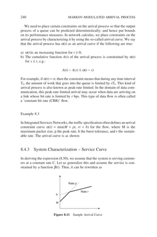
![D t A s t s
A t
s t
( ) inf { ( ) ( )}
( )( )
= + −
= ⊗
−
≤ ≤
0
β
β (8.51)
The ⊗ notation is the so-called convolution operation in min-plus algebra.
The expression resembles the convolution of the input signal function and the
impulse function to yield the output process in system theory, except the min-
plus convolution operation here replaces multiplication with addition, and
addition with the computation of infimum.
This leads us to the definition of the service curve. We say that a system
offers to the input process a service curve b if and only if
D t A t
( ) ( )( )
= ⊗ β (8.52)
From Equation (8.51), we see that given the characterization of arrival
process in terms of arrival curve and the characterization of service process in
terms of service curve, the departing process of a queue can be calculated
deterministically. This is the essence of network calculus.
8.4.4 Min-Plus Algebra
In previous sections, we introduced the notions of infimum and supremum. We
shall clarify these terms here. Students can refer to (Boudec and Thiran 2002)
for more detail.
Conceptually, infimum and supremum are similar to the minimum and
maximum of a set respectively with some minor differences. Consider a non-
empty set S {s ∈S}; it is said to be bounded from below if there is a number
N1 such that s ≥ N1. That number N1 is the infimum of S. If N1 happens to be
an element in set S and is smaller than any other elements in the set, then is
called the minimum of S. For example, the closed and open interval of [a, b]
and (a, b) have the same infimum, but (a, b) does not have a minimum.
Similarly, S is said to be bounded from above if there is a number N2 such
that S ≤ N2, then N2 is the supremum of S. If it happens to be an element in
the set and is larger than any other elements in the set, it is called the maximum
of S. For example, sup [4,5,6] = max [4,5,6] = 6.
In conventional linear system theory, the convolution between two functions
is defined as
(f ⊗ g)(t) = −∞
∞
∫ f(t − s)g(s)ds
However, in min-plus algebra, the usual addition operator is replaced by the
inf (or min) operator and the multiplication operator by the addition operator.
Hence, the convolution of two functions is given as
NETWORK CALCULUS 241](https://image.slidesharecdn.com/qtts-230925120453-047b3b23/85/QTTS-pdf-264-320.jpg)
![242 MARKOV-MODULATED ARRIVAL PROCESS
( )( ) inf [ ( ) ( )]
f g t f s g t s
s t
⊗ = + −
≤ ≤
0
(8.53)
Similar to the conventional convolution, the min-plus convolution is associa-
tive, commutative and distributive as
(f ⊗ g) ⊗ h = f ⊗ (g ⊗ h) Associativity
f ⊗ g = g = g ⊗ f Commutativity
[inf(f, g)] ⊗ h = inf(f ⊗ h, g ⊗ h) Distributivity](https://image.slidesharecdn.com/qtts-230925120453-047b3b23/85/QTTS-pdf-265-320.jpg)
![9
Flow and Congestion Control
Today, we often experience congestion in modern cities, in terms of long
queues of cars, buses and people waiting for services. Congestion is usually
caused by unpredictable events. Although the daily rush hour is semi-predict-
able, congestion can also be random due to breakdowns and accidents that
cause delays and long queues stretching for long distances. Therefore, a control
mechanism might be implemented, such as using traffic lights to delay access
to a junction or by restricting access to crowded areas in central business dis-
tricts through tolls and congestion charges.
In general, the communication network is similar to our everyday experi-
ences and consists of finite resources, such as bandwidth, buffer capacity for
packets and transmission capacity that depend on traffic control mechanisms
to alleviate congestion problems.
There are specific requirement guarantees, referred to as Quality of Service
(QoS), specified for each traffic flow. When the offered traffic load from the
user to the network exceeds the design limit and the required network resources,
congestion will often occur. In this section, we introduce several specific
examples, where queueing theory has been successfully applied to study the
behaviour of the network under these extreme conditions. We describe key
parameters of performances, i.e. throughput g and time delay E[T]. It is impor-
tant to examine the basic functioning of the network, as shown in Figure 9.1.
9.1 INTRODUCTION
The topic of congestion control has a long history (Schwartz 1987). A simple
mechanism for preventing congestion is flow control, which involves
Queueing Modelling Fundamentals Second Edition Ng Chee-Hock and Soong Boon-Hee
© 2008 John Wiley Sons, Ltd](https://image.slidesharecdn.com/qtts-230925120453-047b3b23/85/QTTS-pdf-266-320.jpg)
![244 FLOW AND CONGESTION CONTROL
regulating the arrival rate at which the traffic enters the network cloud, shown
in Figure 9.1. In general, the network layer carries out routing functions in the
network and provides adequate flow control to ensure timely delivery of packets
from source to destination. The flow control protocols studied here are related
to a packet-switched network, and the main functions of flow control are:
• Prevention of throughput and response time degradation, and loss of effi-
ciency due to network and user overload;
• Deadlock avoidance;
• Fair allocation of resources among competing users;
• Speed matching between the network and attached users.
One simple taxonomy (Yang and Reddy 1995) that describes this well is the
defined congestion control as an open and closed congestion control mecha-
nism. The open-loop flow control mechanism is characterized by having no
feedback between the source and the destination node. This control mechanism
requires the allocation of resources with necessary prior reservation before-
hand. However, the open-loop flow control has inherent problems with maxi-
mizing the utilization of the network resources. Resource allocation is made at
connection setup using a CAC (Connection Admission Control) and this alloca-
tion is made using information that is already ‘old news’ during the lifetime of
the connection. Often this process is inefficient and therefore results in over-
allocation of resources.
For example, in ATM networks, the open-loop flow control is used by CBR
(Constant Bit Rate), VBR (Variable Bit Rate) and UBR (Unspecified Bit Rate)
traffic. On the other hand, the closed-loop flow control mechanism is character-
ized by the ability of the network to report pending network congestion back
to the source node. This information is then used by the source node in various
ways to adapt its activity, for example, by slowing down its rate depending on
existing network conditions.
In this chapter, we examine the sliding window and rate-based flow control
mechanism, which is a mathematical abstraction of a closed-loop flow control
End-to-end delay
Arrival rate
Throughput
γ
γ
E[T]
λ
Network cloud
Figure 9.1 Flow control design based on queueing networks](https://image.slidesharecdn.com/qtts-230925120453-047b3b23/85/QTTS-pdf-267-320.jpg)
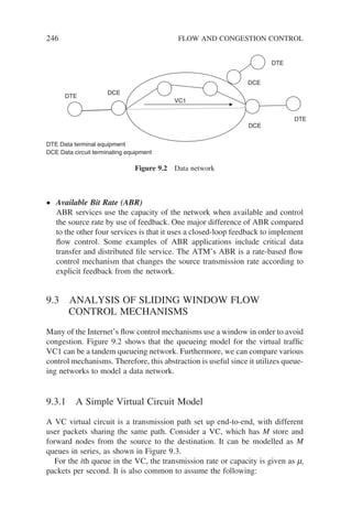
![(i) propagation delay is negligible, and the delay consists of queuing delay
(waiting time) and transmission delay;
(ii) 1/mi at the ith node represents the average time required to transmit a
packet over its outgoing link;
(iii) independence and the packet lengths are exponentially distributed.
These assumptions make the analysis more tractable and lead to a product form
closed queueing network.
9.3.2 Sliding Window Model
The analysis follows [Schwartz 1988] where the sliding window flow control
protocol is often described in the following manner:
(a) Each packet is individually ACKnowledged, when it arrives at the destina-
tion node.
(b) The ACK, on arriving back at the source node, shifts the window forward
by 1.
(c) Packets can be transmitted onto the VC as long as there are fewer than N
(window size) packets along the VC.
(d) Arriving packets are assumed blocked and lost to the system if the window
is depleted (i.e. N outstanding unacknowledged packets).
Suppose we neglect the delay incurred by acknowledgment returning from the
destination end of the VC back to the source end. Hence we have a closed
network, as shown in Figure 9.4 below:
When N packets are in transit along the VC, the bottom queue is empty and
cannot serve (depleted window condition). Once one of the packets arrives at
its destination, it appears in the M + 1 queue and the source can deliver the
packet at a rate of l.
Normally, we will find a trade-off between time delay and throughput.
Firstly, we will introduce a theorem that is useful to analyse this sliding window
queueing network, which is familiar to circuit analysis.
Stage 1 Stage 2 Stage M
Source Destination
λ µ µ
1 2 m
µ
Figure 9.3 Simplified model for a single virtual circuit
ANALYSIS OF SLIDING WINDOW FLOW CONTROL MECHANISMS 247](https://image.slidesharecdn.com/qtts-230925120453-047b3b23/85/QTTS-pdf-270-320.jpg)
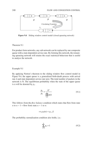
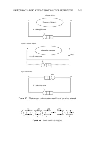
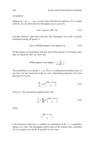
![γ =
=
∑u n pn
n
N
( )
1
(9.7)
We need to apply Little’s formula, which is a general result applicable to
any queue. This states that if a queue has an average customer arrival rate of
l, then the average number of customers N in the queue and the average time
spent by a customer in the queue will be related by N = lW. By Little’s formula,
the end-to-end delay through the VC is
E T
E n
npn
n
[ ]
[ ]
= = = =
average number of packets
end to end throughput γ
1
N
N
∑
γ
(9.8)
Heavy traffic analysis
(i) Let l m, or l → ∞
We note that the upper queue is almost always at state N, i.e. E(n) ≈ N:
γ
µ
= =
− +
u N
N
M N
( )
1
(9.9)
and Little’s theorem:
E T
N M N
[ ] = =
− +
γ µ
1
(9.10)
Figure 9.7 Norton’s equivalent, cyclic queue network
ANALYSIS OF SLIDING WINDOW FLOW CONTROL MECHANISMS 251
N cycling packets
λ
B
A
u(n)
State dependent service rate
n packets
N-n packets](https://image.slidesharecdn.com/qtts-230925120453-047b3b23/85/QTTS-pdf-274-320.jpg)
![252 FLOW AND CONGESTION CONTROL
By combining Equations (9.9) and (9.10), the time delay versus throughput
tradeoffs characteristics are
µ
γ
µ
E T
M
[ ] =
−
−
1
1
(9.11)
As g → m (by increasing N), small changes in g give rise to large changes
in E(T). Various criteria give the value of optimum N, i.e. N = M − 1
(ii) When l = m, (load in the vicinity of the capacity of m of each queue), we
note that there are in effect M + 1 queues instead of M queues (see Figure
9.4):
γ
µ
=
+
N
M N
(9.12)
0.2 0.3 0.4 0.5
γ/µ
0.6 0.7 0.8 0.9
3
4
5
6
7
8
9
10
11
M=3
M=4
8
7
6
5
4
3
2
1
8
7
6
5
4
3
2
1
Sliding Window flow control N=1..8
µE[T]
Figure 9.8 Delay throughput tradeoff curve for sliding window flow control, M = 3,
4 and l → ∞](https://image.slidesharecdn.com/qtts-230925120453-047b3b23/85/QTTS-pdf-275-320.jpg)
![and the new time delay expression:
µE T
M
M
M N
ified to account for M queues
[ ] ( )
mod
=
+
+
+
1
1
(9.13)
The new optimum value of N is
N = M
For the closed queuing network, the product form solution for this type of
network is
p
g N M
i
i
n
i
M i
( )
( , )
n =
=
∏
1
1
λ
µ
(9.14)
g(N, M) is called the normalization constant (statistical parameter of interest).
Note that only ‘relative’ values of li can be found and so ri = li/mi no longer
represents the actual utilization of the ith queue.
Buzen’s Algorithm (Convolution)
g n m g n m g n m
m
( , ) ( , ) ( , )
= − + −
1 1
ρ (9.15)
with initial starting condition:
g n n N
n
( , ) , , , . . . ,
1 0 1 2
1
= =
ρ (9.16)
g m m M
( , ) , , . . . ,
0 1 1 2
= = (9.17)
where
ρ
λ
µ
m
m
m
=
The important desired statistics is contained in the g(N, M) normalization
constant. g(N, M) is also related to the moment generating function. Consider
the number of packets in queueing station i to be equal to or exceed k packets.
Then
Prob /
( ) ( , ) ( , )
n k g N k M g N M
i i
k
≥ = −
ρ (9.18)
ANALYSIS OF SLIDING WINDOW FLOW CONTROL MECHANISMS 253](https://image.slidesharecdn.com/qtts-230925120453-047b3b23/85/QTTS-pdf-276-320.jpg)
![254 FLOW AND CONGESTION CONTROL
Utilization of server: By letting k = 1 in equation (9.18),
Prob Prob
/
( ) ( ) :
( , ) ( , )
n n
g N M g N M
i i
i
≥ = − =
= −
1 1 0
1
ρ (9.19)
Throughput or the average number of packets serviced per unit time for the ith
queue is given as
gi = mi Prob(ni ≥ 1) = mi ri g(N − 1, M)/g(N, M)
= li g(N − 1, M)/g(N, M)
The average number of packets in ith queue is
E n k n k
i i
k
N
[ ] { }
= =
=
∑ Prob
1
Now the marginal probability that queue i has k packets, i.e. Prob(ni = k):
Prob Prob Prob
( ) ( ) ( )
n k n k n k
i i i
= = ≥ − ≥ +1 (9.21)
Substitution for the above and simplifying gives
E n g N k M g N M
i i
k
k
N
[ ] ( , ) ( , )
= −
=
∑ρ /
1
(9.22)
Example 9.2
Consider the following virtual circuit from node 1 to node 4 for packet-
switching network transmission rates (m, 2m, 3m packets/s) for the links, as
indicated in Figure 9.9. Assume that the packet arrivals to this virtual circuit
are a Poisson arrival process with a rate of l packets/s:
(a) Show and explain how the sliding window flow control mechanism for
packet-switched networks can be represented in terms of a network of M/
M/1 queues.
(b) With a window size of N = 1, . . . , 5 for the sliding window flow control
mechanism for this virtual circuit, use Buzen’s algorithm to find the end-
to-end time delay and throughput for l 3 m.](https://image.slidesharecdn.com/qtts-230925120453-047b3b23/85/QTTS-pdf-277-320.jpg)
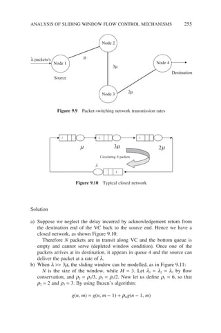
![256 FLOW AND CONGESTION CONTROL
With initial starting condition:
g(n, 1) = r1
n
n = 0, 1, 2, . . . , N
g(0, m) = 1 m = 1, 2, . . . , M where ρ
λ
µ
m
m
m
=
One possible G(n, m) is computed in Table 9.2 below:
The end-to-end throughput can be obtained from
γ µ ρ λ
i i i i
g N M
g N M
g N M
g N M
=
−
=
−
( , )
( , )
( , )
( , )
1 1
which simplifies to
=
−
6
1 3
3
g N
g N
( , )
( , )
The mean number of packets at each queue can be obtained by
E n
g N k M
g N M
i i
k
k
N
[ ]
( , )
( , )
=
−
=
∑ρ
1
1 3
2
µ
3
µ
Circulating N packets
µ
2
Figure 9.11 Sliding window closed network
Table 9.2 Computation of G(n, m)
r 6 2 3
m
n
1 2 3
0 1 1 1
1 6 8 11
2 36 52 85
3 216 320 575
4 1,296 1,936 3,661
5 7,776 11,648 22,631](https://image.slidesharecdn.com/qtts-230925120453-047b3b23/85/QTTS-pdf-279-320.jpg)
![The delay over each of the virtual circuits can be determined by Little’s
formula:
T T
E n
g N k g N
i
i
M
i
i
i
k
k
N
i
i
= = =
−
=
=
=
=
∑
∑
∑
∑
1
1
1
3
1
3
3 3
[ ]
( , ) ( , )
γ
ρ
γ
/
When l 3m, it is obvious that it is not necessary to calculate the numerator
term as it is
E[n] = N
the window size. So the normalized end-to-end throughput and delay can
be calculated as a function of the different window size N, as shown in
Table 9.3:
9.4 RATE BASED ADAPTIVE
CONGESTION CONTROL
For the ATM network, the ABR service will systematically and dynamically
allocate available bandwidths to users by controlling the rate of offered traffic
through feedback. The aim of the ABR service is to support applications with
vague requirements for throughput and delay. Due to these vague requirements,
they are best expressed as ranges of acceptable values. The ABR service allows
a user to specify the lower and upper bound on the bandwidth allotted upon
connection. The control mechanism is based on feedback from the network to
the traffic source.
The ability for the ABR service to work in a variety of environments, i.e.
LANs, MANs or WANs, is particularly important when traffic is controlled
using feedback. The motivation for feedback congestion control is based on
adaptive control theory. A simple model may be derived to control the source
rate l(t) to optimize a particular objective, such as the throughput or stability.
By providing information regarding the buffer occupancy of the bottleneck
queue, we can adjust the rate accordingly. The reader is advised to refer to
advanced textbooks on the subject, such as (McDysan 2000).
Table 9.3 Normalized end-to-end throughput and delay
N 1 2 3 4 5
g /m 0.545 0.776 0.887 0.942 0.971
mT 1.834 2.577 3.382 4.246 5.149
RATE BASED ADAPTIVE CONGESTION CONTROL 257](https://image.slidesharecdn.com/qtts-230925120453-047b3b23/85/QTTS-pdf-280-320.jpg)