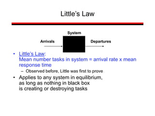
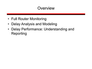
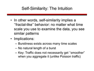
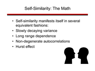
This document provides a summary of concepts in queuing theory and network traffic analysis. It discusses queuing theory concepts like Little's Law, M/M/1 queues, and Kendall's notation. It then covers an empirical study of router delay that models delays using a fluid queue and reports on busy period metrics. Finally, it discusses the concept of network traffic self-similarity found in measurements of Ethernet LAN traffic.

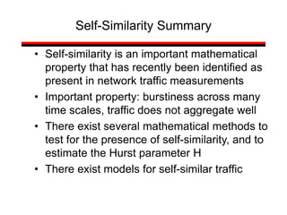
![Introduction
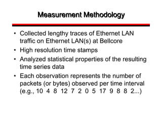
• A classic measurement study has shown that
aggregate Ethernet LAN traffic is self-similar
[Leland et al 1993]
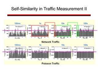
• A statistical property that is very different from
the traditional Poisson-based models
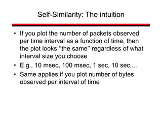
• This presentation: definition of network traffic
self-similarity, Bellcore Ethernet LAN data,
implications of self-similarity](https://image.slidesharecdn.com/queuing-240225071706-d093e123/85/Queuing-theory-and-traffic-analysis-in-depth-57-320.jpg)

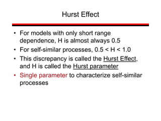
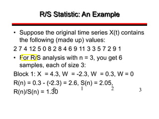
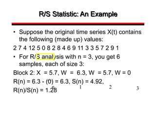
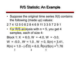
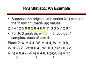
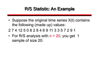
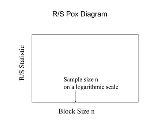
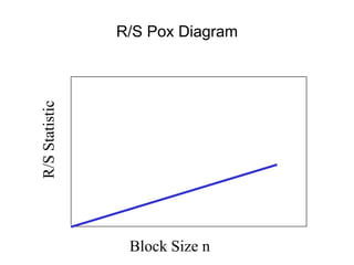
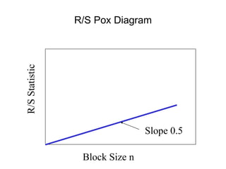
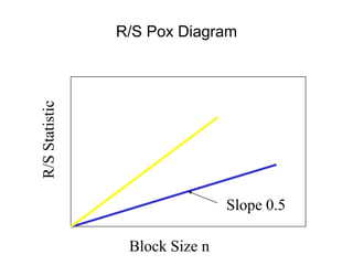
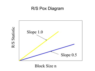
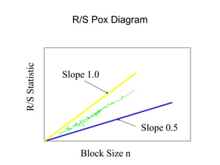
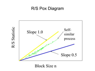
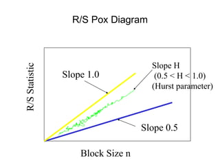
![• For almost all naturally occurring time series,
the rescaled adjusted range statistic (also
called the R/S statistic) for sample size n
obeys the relationship
E[R(n)/S(n)] = c nH
where:
R(n) = max(0, W1, ... Wn) - min(0, W1, ... Wn)
S2(n) is the sample variance, and
for k = 1, 2, ... n
Hurst Effect](https://image.slidesharecdn.com/queuing-240225071706-d093e123/85/Queuing-theory-and-traffic-analysis-in-depth-113-320.jpg)