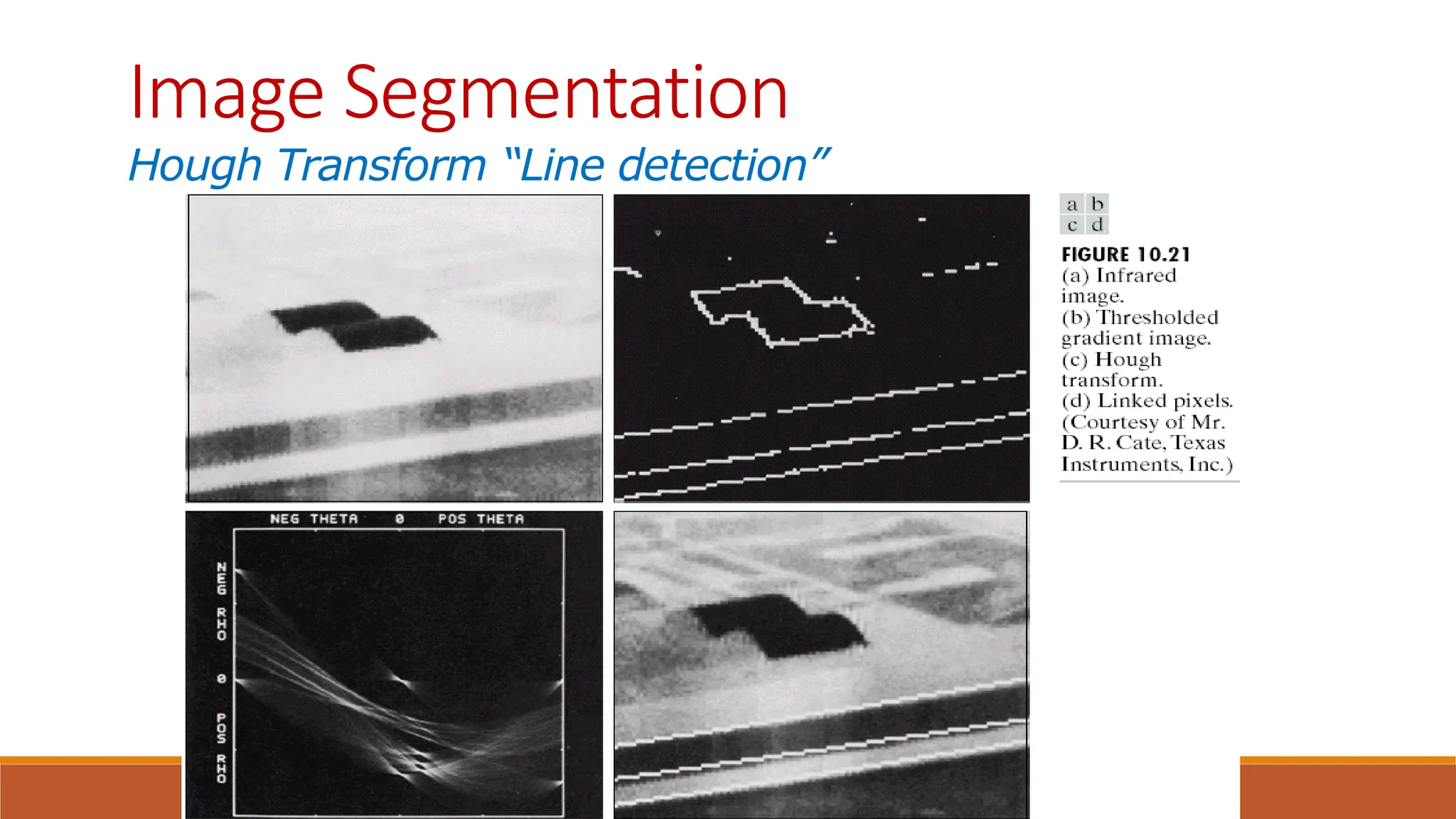
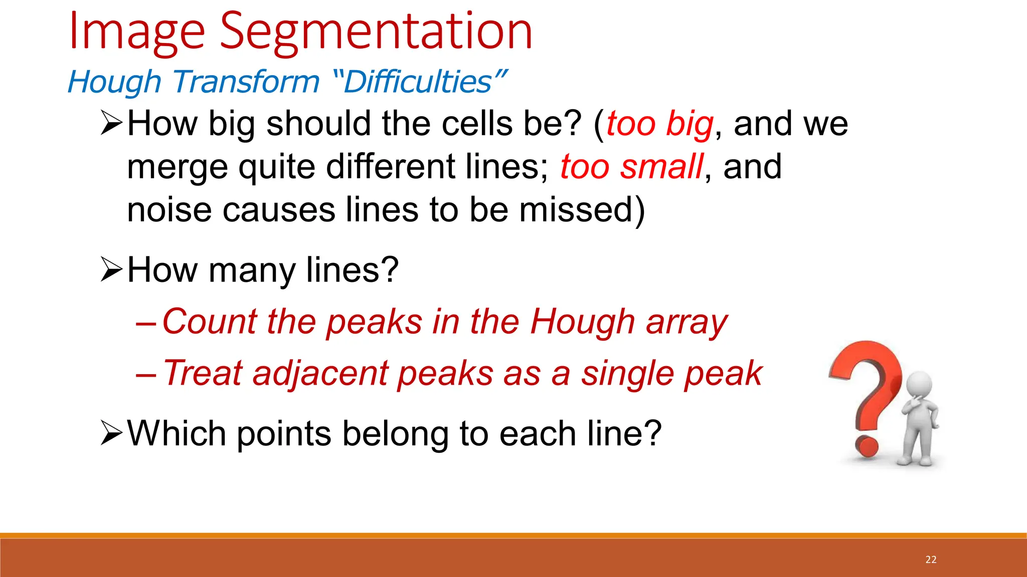
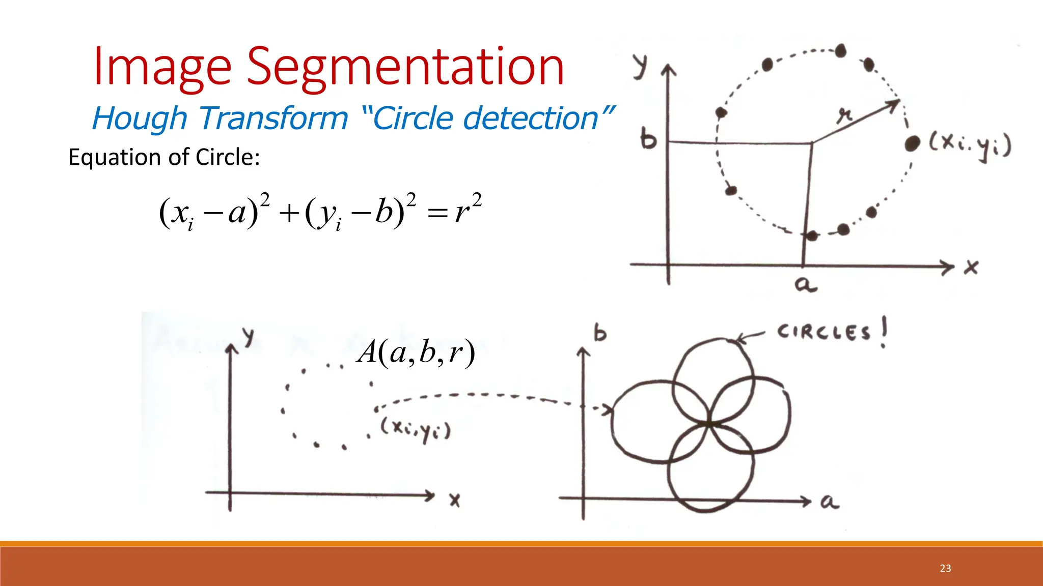
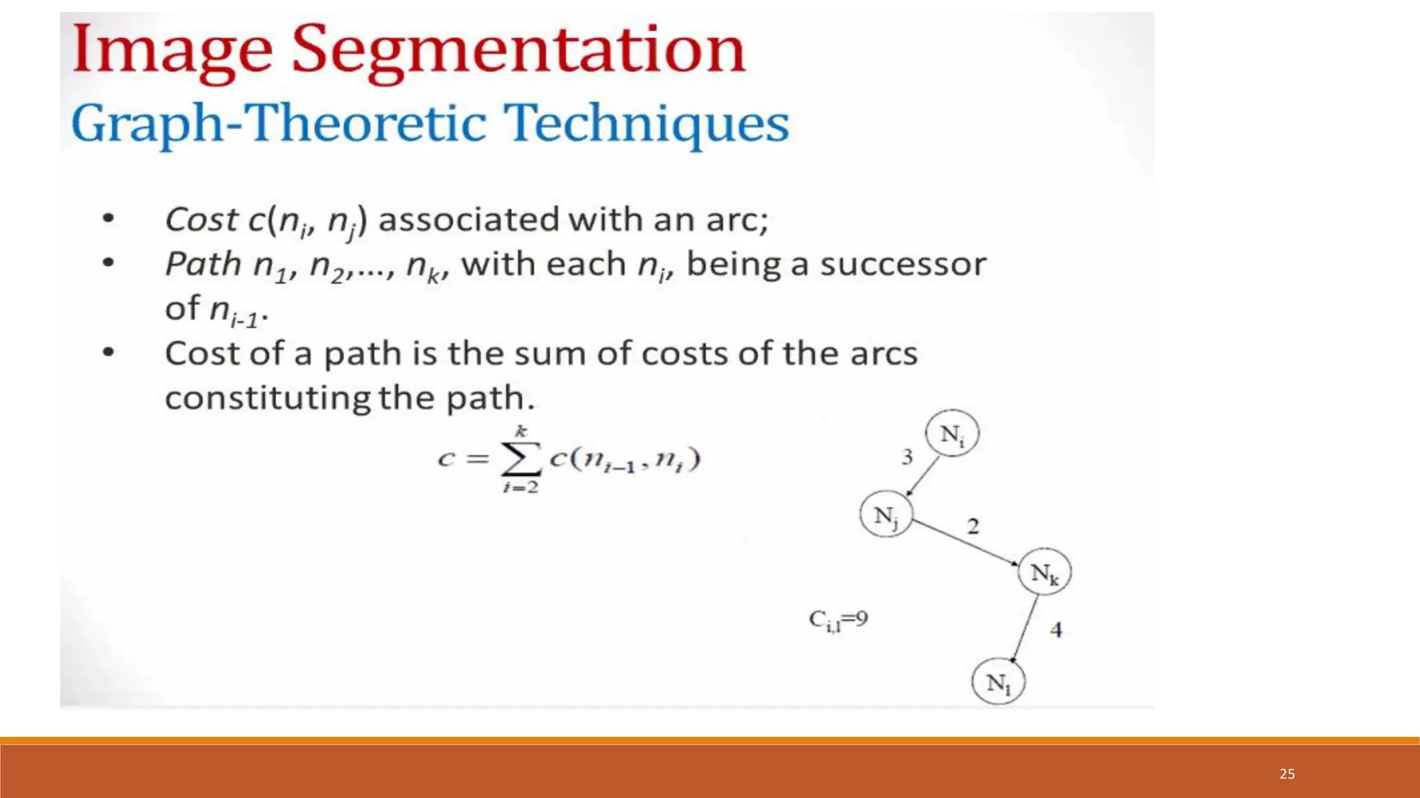
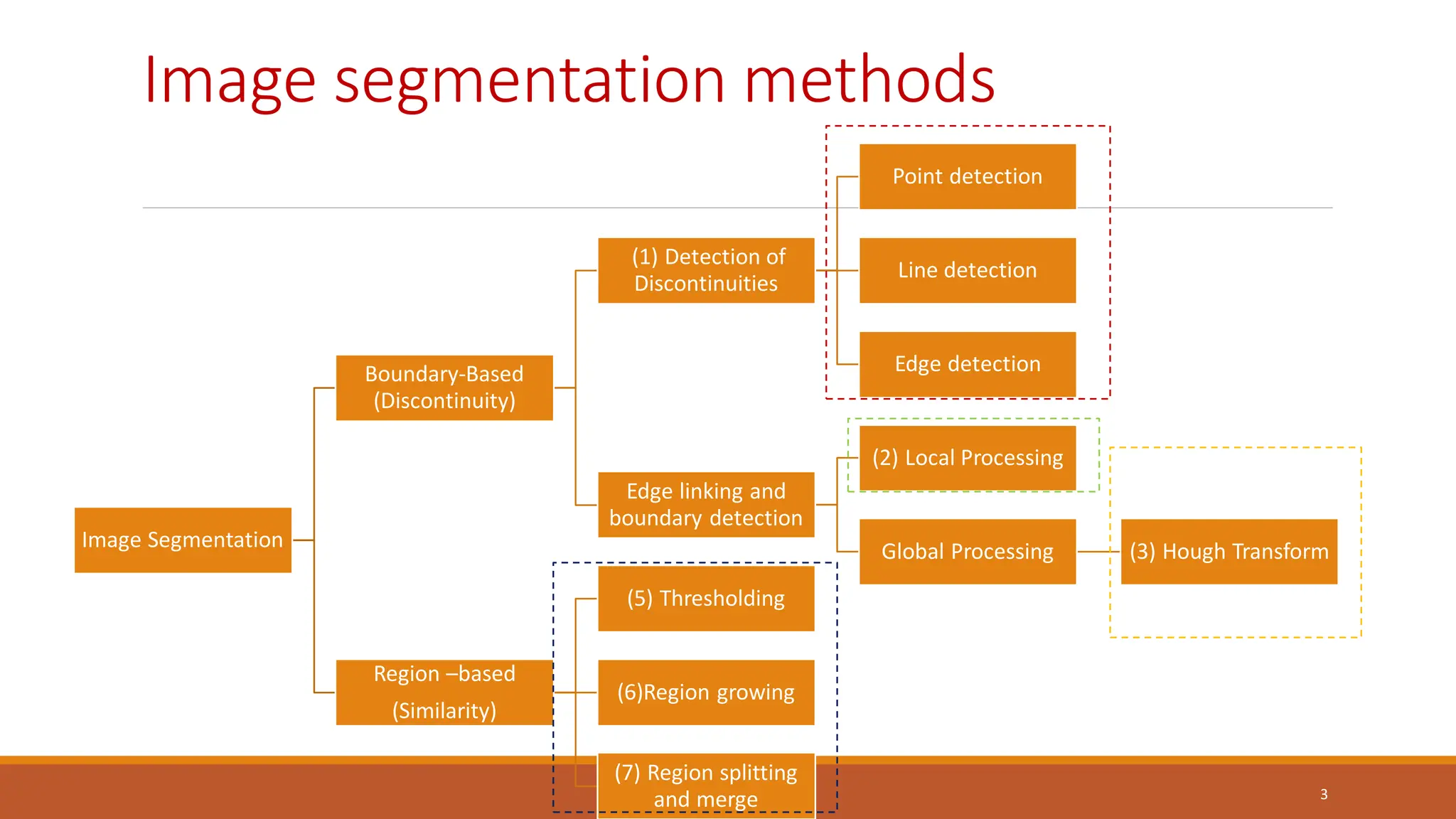
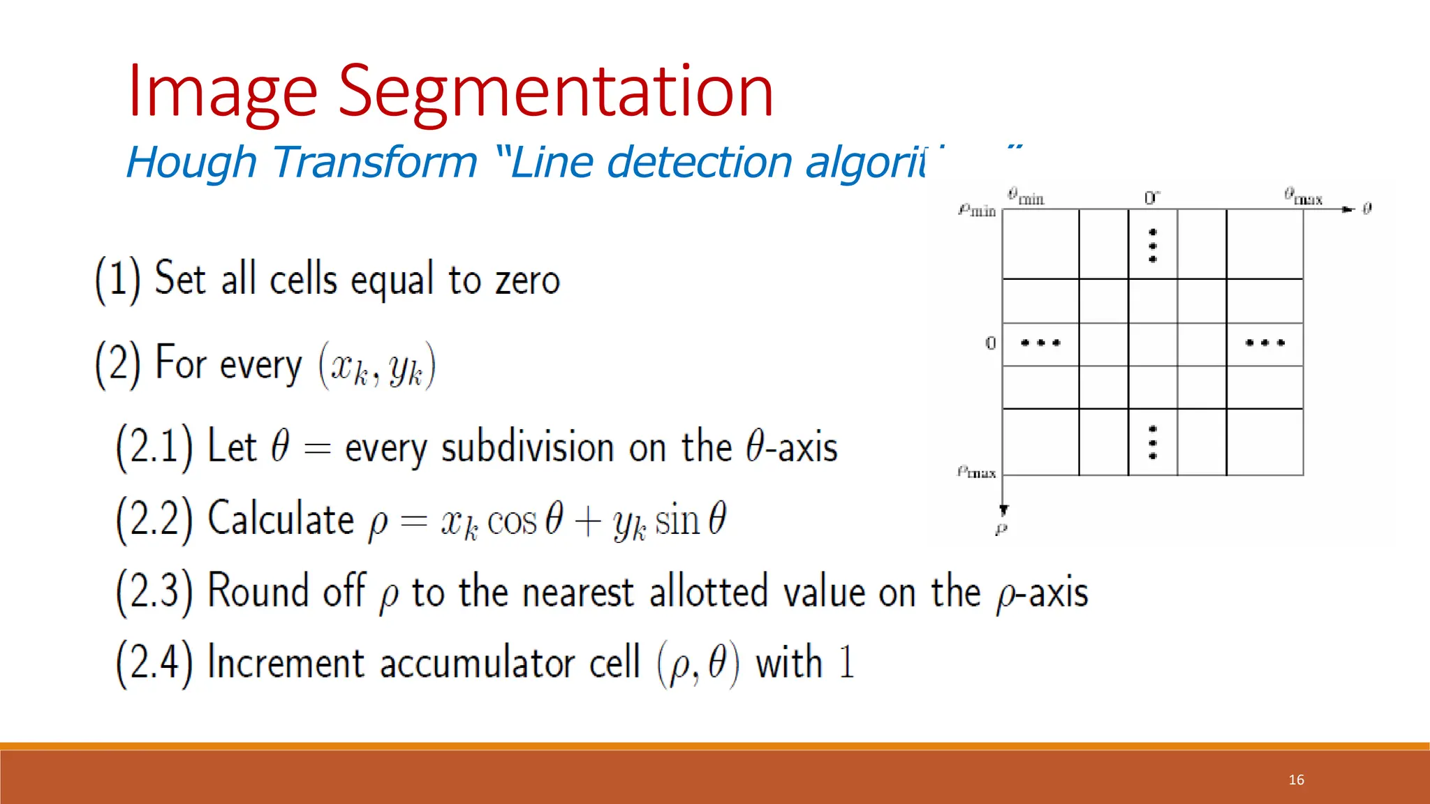
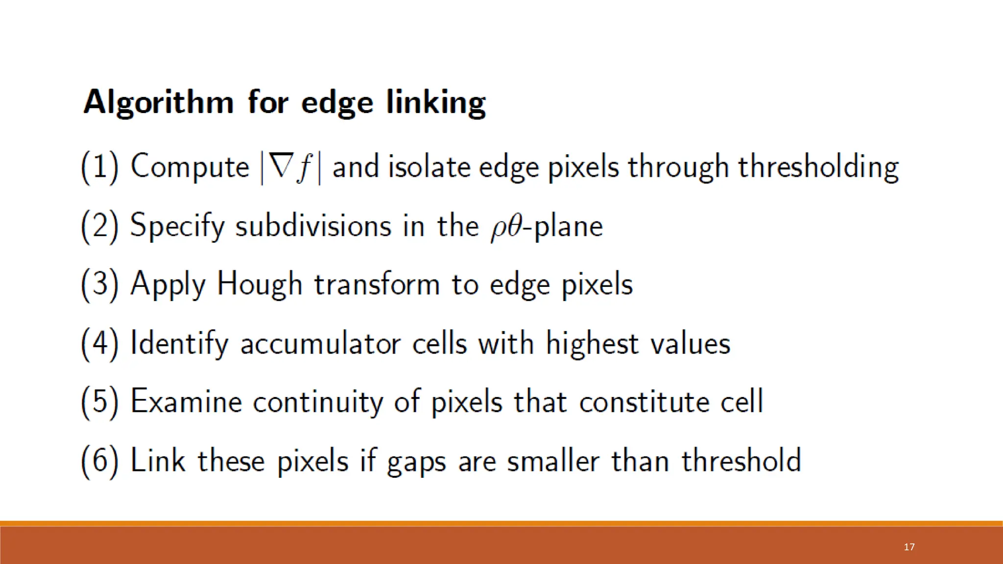
The document discusses image segmentation techniques, particularly focusing on boundary detection and edge linking methods such as local processing and the Hough transform. It explains how edge points are identified and linked using properties like strength and direction. Additionally, it covers the Hough transform for line detection, its algorithmic approach, and challenges associated with effective line and circle detection.

1. Digital Image processing
Assoc. Prof. Elham Shawky Salama Omer
Faculty of Computers, and Artificial Intelligence
Cairo University - Egypt.

2. Image Segmentation
Part-2 “Boundary detection and
Edge Linking”
2

3. Image segmentation methods
Image Segmentation
Boundary-Based
(Discontinuity)
(1) Detection of
Discontinuities
Point detection
Line detection
Edge detection
Edge linking and
boundary detection
(2) Local Processing
Global Processing (3) Hough Transform
Region –based
(Similarity)
(5) Thresholding
(6)Region growing
(7) Region splitting
and merge 3

4. Edge Linking and Boundary Detection
Local Processing
Two properties of edge points are useful for edge linking:
◦ the strength (or magnitude) of the detected edge points
◦ their directions (determined from gradient directions)
This is usually done in local neighborhoods.
Adjacent edge points with similar magnitude and direction
are linked.
For example, an edge pixel with coordinates (x0,y0) in a
predefined neighborhood of (x,y) is similar to the pixel at (x,y)
if
4
threshold
e
nonnegativ
a
:
,
)
,
(
)
,
( 0
0 E
E
y
x
y
x
f 



threshold
angle
nonegative
a
:
,
)
,
(
)
,
( 0
0 A
A
y
x
y
x 



5. Edge Linking and Boundary Detection
Local Processing: Example
In this example, we can
find the license plate
candidate after edge
Linking process.

6. Example-3
Compute the gradient magnitude and angle of the following image using Sobel masks. Apply the
local edge criteria
6
2 3 1 5
6 0 8 2
5 6 7 1

7. Edge Linking and Boundary Detection
Local Processing
1- Apply dx
2- Apply dy
3- Apply
4- Apply threshold on
5- For every one value (e.g. =1) in matrix 4
7
 2
1
2
2
)
(
mag y
x G
G
f 



 f
1
( , ) tan
y
x
G
x y
G
   
  
 
f

threshold
e
nonnegativ
a
:
,
)
,
(
)
,
( 0
0 E
E
y
x
y
x
f 



threshold
angle
nonegative
a
:
,
)
,
(
)
,
( 0
0 A
A
y
x
y
x 



8. Thr. For mag.=4, Thr. For dir.=2
0 0 0 0
1 0 0 0
1 1 1 1
8
14 13 1 1
18 12 11 24
16 15 19 25
1.1 -1.5 1.2 -0.8
0.7 1.2 1.4 0.0
8
-0.7 -1.2 1.1 0.5
f
 ( , )
x y

• For example pixel pos(1,0) with value 1
• |18-14|=4 <=4 (yes) |0.7-1.1|=-0.4 <2 (Yes)
(Yes&Yes ) zero became 1
• |18-13|=5 <=2 (NO) |0.7+1.5|=2.2<2 (NO)
(No&No) zero still zero
• |18-12|=6 <2 (No) |0.7-1.2|=1.9<2 (Y)
(No&Yes) zero still zero
Threshold Matrix

9. Image segmentation methods
Image Segmentation
Boundary-Based
(Discontinuity)
(1) Detection of
Discontinuities
Point detection
Line detection
Edge detection
Edge linking and
boundary detection
(2) Local Processing
Global Processing (3) Hough Transform
Region –based
(Similarity)
(5) Thresholding
(6)Region growing
(7) Region splitting
and merge 9

10. Image Segmentation
Hough Transform “Line detection”
10
Hough transform: a way of finding edge points in an image that
lie along a straight line.
◦ IDEA: xy-plane v.s. ab-plane (parameter space)

11. Image Segmentation
Hough Transform “Line detection”
11
j j
j j
y ax b or
b x a y
 
  
( , )
j j
x y
)
,
( i
i y
x
i i
i i
y ax b or
b x a y
 
  
Equation of Line:
Find:
y ax b
 
( , )
a b

12. 12
y ax b
 
)
,
( i
i y
x
y
x
a
b
( , )
a b
Image Space
Parameter Space
Parameter space also called Hough Space
Image Segmentation
Hough Transform “Line detection”
x,y plan

13. Since the equation
has infinite slope for the vertical line, We introduced a singularity-free alternative, the line
parametrization
13


 
 sin
cos y
x
b
ax
y i
i 
 i i
b x a y
  
max
0
2
0








Image Segmentation
Hough Transform “Line detection”
2D
  
where D is the distance between
corners in the image

14. The Hough transform consists of
finding all pairs of values of  and 
which satisfy the equations that
pass through (x,y).
These are accumulated in what is
basically a 2-dimensional histogram.
When plotted these pairs of  and
 will look like a sine wave. The
process is repeated for all
appropriate (x,y) locations.


 
 sin
cos y
x
Image Segmentation
Hough Transform “Line detection”

15. The intersection of the
curves corresponding
to points 1,3,5
2,3,4
1,4
Image Segmentation
Hough Transform “Line detection”

16. 16
Image Segmentation
Hough Transform “Line detection algorithm”

17. 17

18. 18
Hough Transform Example
Solve to get Hough transform using four quantization levels
for the angles from 0 to π and five uniform quantization levels
of the radial distance from 0 to the maximum distance , Use a
threshold of 3 to detect strong lines in the image
0 0 1 1 0
0 0 0 1 0
0 0 0 1 0
0 0 0 0 1

19. 19
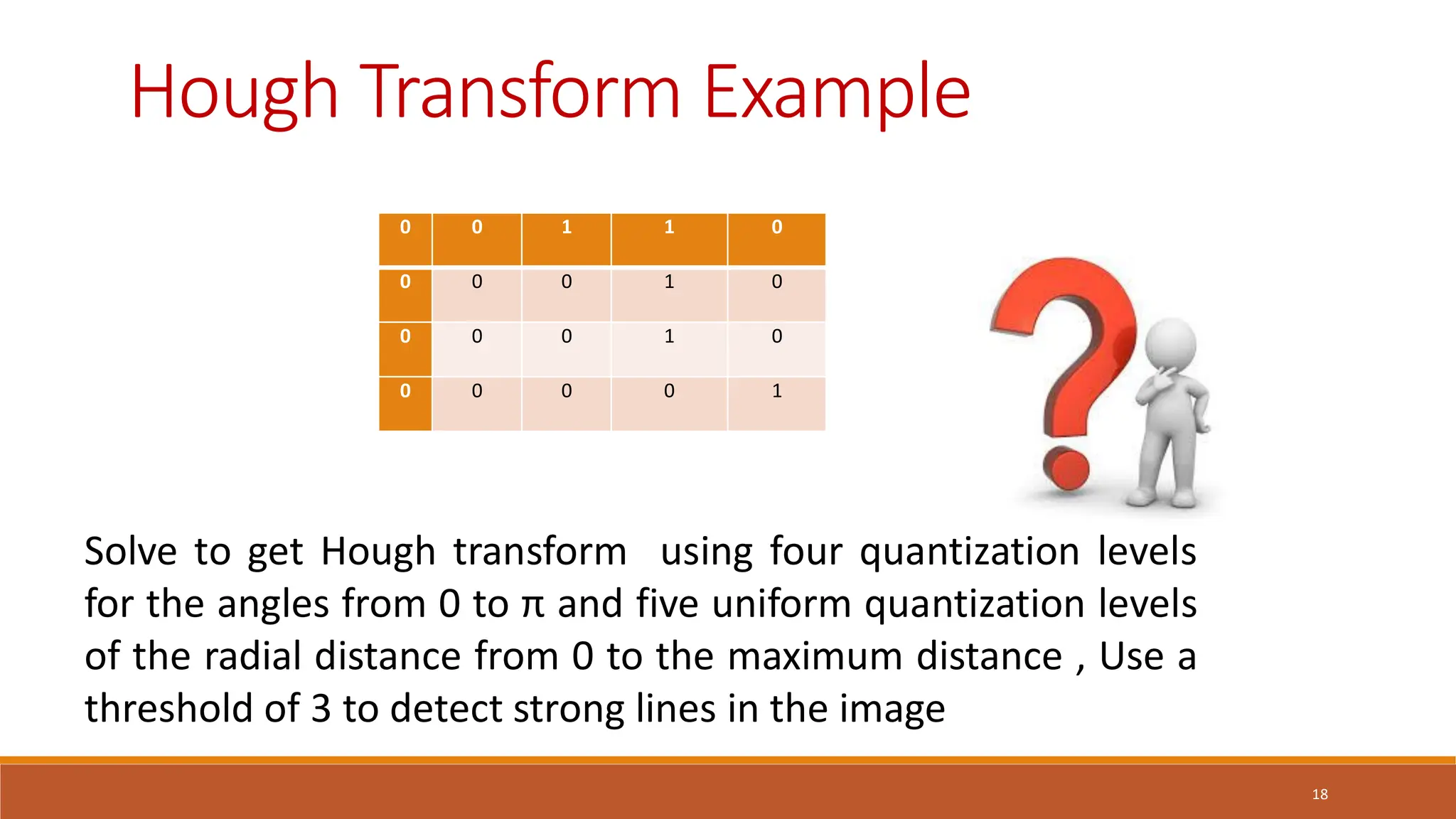
ϴ=[0,𝜋], 4 levels
ϴ =[0,
𝜋
4
,
𝜋
2
,
3𝜋
4
, 𝜋]
=[0,max _𝑑𝑖𝑠𝑡𝑎𝑛𝑐𝑒]=[0,𝐷], 5 levels
D=[(0,0),(3,4)]= 9 + 16 = 5
ϴ =[0,1,2,3,4,5]
0
1
2
3
4
5
4
 2
4
 3
4
 4
4



0 0 1 1 0
0 0 0 1 0
0 0 0 1 0
0 0 0 0 1
First Index: (0,2), x=0,y=2


20. 20
0
0 2 3 1
1 6 1
2
2[0,2],[0,4
]
5 0
3 1 8 4
4 9
5
4
 2
4
 3
4
 4
4



First Index: (0,3), x=0,y=3
ϴ =0 ϴ =
𝜋
4
ϴ =
𝜋
2
ϴ =
3𝜋
4
ϴ =𝜋
=(0)𝑐𝑜𝑠(0)+3sin(0)=0 =(0)𝑐𝑜𝑠(
𝜋
4
)+3si
n(
𝜋
4
)=3
=(0)𝑐𝑜𝑠(
𝜋
2
)+
2sin(
𝜋
2
)=2 =(0)𝑐𝑜𝑠(
3𝜋
4
)+
2sin(
3𝜋
)=3
=
(0)𝑐𝑜𝑠(𝜋)
+2sin(𝜋)
=0
= 𝑥𝑐𝑜𝑠ϴ+ysinϴ
   



21. Image Segmentation
Hough Transform “Line detection”

22. 22
How big should the cells be? (too big, and we
merge quite different lines; too small, and
noise causes lines to be missed)
How many lines?
–Count the peaks in the Hough array
–Treat adjacent peaks as a single peak
Which points belong to each line?
Image Segmentation
Hough Transform “Difficulties”

23. 23
Equation of Circle:
2
2
2
)
(
)
( r
b
y
a
x i
i 



)
,
,
( r
b
a
A
Image Segmentation
Hough Transform “Circle detection”

24. 24

25. 25

26. 26

27. 27

28. 28

29. 29

30. 30

31. 31

32. 32

33. 33

34. 34

35. 35

36. 36