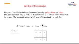
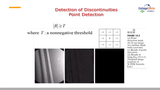
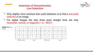
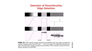
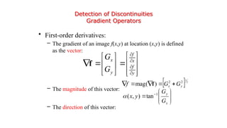
Program : B. Tech (AI& ML)
Digital Image Processing
• Region based Segmentation,
UNIT 03 : Topic 4
• Split and Merge Technique
UNIT 03 : Topic 5
• Image Representation and Description
UNIT 03 : Topic 6
• Chain Code, Polygonal
UNIT 03 : Topic 7
• Representation, Shape Number, Moments
UNIT 03 : Topic 8
• Detection of Discontinuities,
UNIT 03 : Topic 1
• Edge Linking using Hough Transform,
UNIT 03 : Topic 2
• Thresholding
UNIT 03 : Topic 3
• Detection of Discontinuities
UNIT 03 :
Topic 1
Introduction
Image segmentation divides an image into regions that are connected and have some
similarity within the region and some difference between adjacent regions.
The goal is usually to find individual objects in an image.
For the most part there are fundamentally two kinds of approaches to segmentation:
discontinuity and similarity.
Similarity may be due to pixel intensity, color or texture.
Differences are sudden changes (discontinuities) in any of these, but especially sudden changes in
intensity along a boundary line, which is called an edge.
Detection of Discontinuities
There are three kinds of discontinuities of intensity: points, lines and edges.
The most common way to look for discontinuities is to scan a small mask over
the image. The mask determines which kind of discontinuity to look for.







9
1
9
9
2
2
1
1 ...
i
i
i z
w
z
w
z
w
z
w
R
Detection of Discontinuities
Line Detection
• Only slightly more common than point detection is to find a one pixel
wide line in an image.
• For digital images the only three point straight lines are only
horizontal, vertical, or diagonal (+ or –45).
Detection of Discontinuities
Line Detection
Detection of Discontinuities
Edge Detection
Detection of Discontinuities
Edge Detection
Detection of Discontinuities
Edge Detection
Detection of Discontinuities
Edge Detection
Detection of Discontinuities
Gradient Operators
• First-order derivatives:
– The gradient of an image f(x,y) at location (x,y) is defined
as the vector:
– The magnitude of this vector:
– The direction of this vector:





















y
f
x
f
y
x
G
G
f
 2
1
2
2
)
(
mag y
x G
G
f 



 f








 
x
y
G
G
y
x 1
tan
)
,
(

Detection of Discontinuities
Gradient Operators
Roberts cross-gradient operators
Prewitt operators
Sobel operators
Detection of Discontinuities
Gradient Operators
Prewitt masks for
detecting diagonal edges
Sobel masks for
detecting diagonal edges
y
x G
G
f 


Detection of Discontinuities
Gradient Operators: Example
Detection of Discontinuities
Gradient Operators: Example
Detection of Discontinuities
Gradient Operators: Example
Detection of Discontinuities
Gradient Operators
• Second-order derivatives: (The Laplacian)
– The Laplacian of an 2D function f(x,y) is defined as
– Two forms in practice:
2
2
2
2
2
y
f
x
f
f







Detection of Discontinuities
Gradient Operators
• Consider the function:
• The Laplacian of h is
• The Laplacian of a Gaussian sometimes is called the Mexican
hat function. It also can be computed by smoothing the image
with the Gaussian smoothing mask, followed by application of
the Laplacian mask.
deviation
standard
the
:
and
where
)
( 2
2
2
2 2
2


y
x
r
e
r
h
r





2
2
2
4
2
2
2
)
( 


r
e
r
r
h






 



The Laplacian of a
Gaussian (LoG)
A Gaussian function
Detection of Discontinuities
Gradient Operators
Detection of Discontinuities
Gradient Operators: Example
Sobel gradient
Laplacian mask
Gaussian smooth function
Edge Linking and Boundary Detection
Local Processing
• Two properties of edge points are useful for edge linking:
– the strength (or magnitude) of the detected edge points
– their directions (determined from gradient directions)
• This is usually done in local neighborhoods.
• Adjacent edge points with similar magnitude and direction are
linked.
• For example, an edge pixel with coordinates (x0,y0) in a
predefined neighborhood of (x,y) is similar to the pixel at (x,y)
if
threshold
e
nonnegativ
a
:
,
)
,
(
)
,
( 0
0 E
E
y
x
y
x
f 



threshold
angle
nonegative
a
:
,
)
,
(
)
,
( 0
0 A
A
y
x
y
x 
 

Edge Linking and Boundary Detection
Local Processing: Algorithm
1. Compute the gradient magnitude and angle arrays, M(x, y) and α(x, y),
of the input image, f(x, y).
2. Form a binary image, g(x, y), whose value at any pair of coordinates (x,
y) is given by:
where TM is a threshold, A is a specific angle direction, and ±TA defines a
“band” of acceptable direction about A.
3. Scan the rows of g and fill all gaps in each row that do not exceed a
specified length, K.
4. To detect gaps in other direction, θ, rotate g by this angle and apply the
horizontal scanning procedure in step 3. Rotate the result back by –θ.
1, ( , ) AND ( , )
( , )
0, Otherwise
M A
M x y T x y A T
g x y

  



Edge Linking and Boundary Detection
Local Processing: Example
In this example,
we can find the
license plate
candidate after
edge linking
process.
Digital Image Processing -Unit-3 - L1.pptx

Digital Image Processing -Unit-3 - L1.pptx

  • 1.
    Program : B.Tech (AI& ML) Digital Image Processing
  • 2.
    • Region basedSegmentation, UNIT 03 : Topic 4 • Split and Merge Technique UNIT 03 : Topic 5 • Image Representation and Description UNIT 03 : Topic 6 • Chain Code, Polygonal UNIT 03 : Topic 7 • Representation, Shape Number, Moments UNIT 03 : Topic 8 • Detection of Discontinuities, UNIT 03 : Topic 1 • Edge Linking using Hough Transform, UNIT 03 : Topic 2 • Thresholding UNIT 03 : Topic 3
  • 3.
    • Detection ofDiscontinuities UNIT 03 : Topic 1
  • 4.
    Introduction Image segmentation dividesan image into regions that are connected and have some similarity within the region and some difference between adjacent regions. The goal is usually to find individual objects in an image. For the most part there are fundamentally two kinds of approaches to segmentation: discontinuity and similarity. Similarity may be due to pixel intensity, color or texture. Differences are sudden changes (discontinuities) in any of these, but especially sudden changes in intensity along a boundary line, which is called an edge.
  • 5.
    Detection of Discontinuities Thereare three kinds of discontinuities of intensity: points, lines and edges. The most common way to look for discontinuities is to scan a small mask over the image. The mask determines which kind of discontinuity to look for.        9 1 9 9 2 2 1 1 ... i i i z w z w z w z w R
  • 7.
    Detection of Discontinuities LineDetection • Only slightly more common than point detection is to find a one pixel wide line in an image. • For digital images the only three point straight lines are only horizontal, vertical, or diagonal (+ or –45).
  • 8.
  • 9.
  • 10.
  • 11.
  • 12.
  • 13.
    Detection of Discontinuities GradientOperators • First-order derivatives: – The gradient of an image f(x,y) at location (x,y) is defined as the vector: – The magnitude of this vector: – The direction of this vector:                      y f x f y x G G f  2 1 2 2 ) ( mag y x G G f      f           x y G G y x 1 tan ) , ( 
  • 14.
    Detection of Discontinuities GradientOperators Roberts cross-gradient operators Prewitt operators Sobel operators
  • 15.
    Detection of Discontinuities GradientOperators Prewitt masks for detecting diagonal edges Sobel masks for detecting diagonal edges
  • 16.
    y x G G f    Detectionof Discontinuities Gradient Operators: Example
  • 17.
  • 18.
  • 19.
    Detection of Discontinuities GradientOperators • Second-order derivatives: (The Laplacian) – The Laplacian of an 2D function f(x,y) is defined as – Two forms in practice: 2 2 2 2 2 y f x f f       
  • 20.
    Detection of Discontinuities GradientOperators • Consider the function: • The Laplacian of h is • The Laplacian of a Gaussian sometimes is called the Mexican hat function. It also can be computed by smoothing the image with the Gaussian smoothing mask, followed by application of the Laplacian mask. deviation standard the : and where ) ( 2 2 2 2 2 2   y x r e r h r      2 2 2 4 2 2 2 ) (    r e r r h            The Laplacian of a Gaussian (LoG) A Gaussian function
  • 21.
  • 22.
    Detection of Discontinuities GradientOperators: Example Sobel gradient Laplacian mask Gaussian smooth function
  • 23.
    Edge Linking andBoundary Detection Local Processing • Two properties of edge points are useful for edge linking: – the strength (or magnitude) of the detected edge points – their directions (determined from gradient directions) • This is usually done in local neighborhoods. • Adjacent edge points with similar magnitude and direction are linked. • For example, an edge pixel with coordinates (x0,y0) in a predefined neighborhood of (x,y) is similar to the pixel at (x,y) if threshold e nonnegativ a : , ) , ( ) , ( 0 0 E E y x y x f     threshold angle nonegative a : , ) , ( ) , ( 0 0 A A y x y x    
  • 24.
    Edge Linking andBoundary Detection Local Processing: Algorithm 1. Compute the gradient magnitude and angle arrays, M(x, y) and α(x, y), of the input image, f(x, y). 2. Form a binary image, g(x, y), whose value at any pair of coordinates (x, y) is given by: where TM is a threshold, A is a specific angle direction, and ±TA defines a “band” of acceptable direction about A. 3. Scan the rows of g and fill all gaps in each row that do not exceed a specified length, K. 4. To detect gaps in other direction, θ, rotate g by this angle and apply the horizontal scanning procedure in step 3. Rotate the result back by –θ. 1, ( , ) AND ( , ) ( , ) 0, Otherwise M A M x y T x y A T g x y       
  • 25.
    Edge Linking andBoundary Detection Local Processing: Example In this example, we can find the license plate candidate after edge linking process.

Editor's Notes

  • #4 Real world is continuous – an image is simply a digital approximation of this.
  • #5 Real world is continuous – an image is simply a digital approximation of this.
  • #6 Real world is continuous – an image is simply a digital approximation of this.
  • #7 Real world is continuous – an image is simply a digital approximation of this.
  • #8 Real world is continuous – an image is simply a digital approximation of this.