See discussions, stats,and author profiles for this publication at: https://www.researchgate.net/publication/286582273
Implementation of Hough Transform for image processing applications
Conference Paper · April 2014
DOI: 10.1109/ICCSP.2014.6949962
CITATIONS
20
READS
311
2 authors, including:
Chandrasekar Lakshumanan
GlobalFoundries Inc.
20 PUBLICATIONS 103 CITATIONS
SEE PROFILE
All content following this page was uploaded by Chandrasekar Lakshumanan on 19 July 2022.
The user has requested enhancement of the downloaded file.
extraneous noise andperforms line detection even when the
lines in the image contain gaps. Once all the points in an
image are transformed using this method, the Hough
parameter space can be inspected for local maxima which
indicate the orientation and the position of the straight lines in
the original image. The Hough accumulator array thus serves
as an indicator of the exact position of the straight line in the
image. The main drawbacks of DA are its high memory
requirements and computational complexity, and these impose
a limitation on the use of the transform for real-time
applications. However, the transform is computationally
expensive and the standard form is ineffective for real-time
segmentation applications.
Line detection [5] is often needed in computer vision
applications. The Hough transform processing of image data
for line detection is robust but time-consuming. With the use
of multiple processors, the processing time for Hough
transform can be much reduced. The Hough transform needs
accumulator memory to store the voting count in each
probable parameter point. It could obtain a point in the
parameter space by a single accumulation. However, all of the
pixels in the binary feature image need to go through the
computation pixel by pixel, which limits its throughput.
III. DETAILED STUDY OF HOUGH TRANSFORM
The Hough Transform is used for the detection of features
of a particular shape like lines or circles in digitalized images.
The Hough transform has long been recognized as a robust
technique for detecting multi-dimensional features in an image
and estimating their parameters. It has many applications, as
most manufactured parts contain feature boundaries, which
can be described by regular curves or straight lines. Its main
advantage is that it is tolerant of gaps in feature boundary
descriptions and is relatively unaffected by noisy image.
The purpose of the technique is to fmd imperfect instances
of objects within a certain class of shapes by a voting
procedure. This voting procedure is carried out in a parameter
space, from which object candidates are obtained as local
maxima in a accumulator space that is explicitly constructed
by the algorithm for computing the Hough transform. It
transforms between the Cartesian space and a parameter space
in which a straight line can be defmed [6]. Let's consider the
case where we have straight lines in an image. We first note
that for every point (Xi, Yi) in that image, all the straight lines
passing through that point satisfy (1) for varying values of line
slope and intercept (m, c).
Yi = mXi + C (1)
Now if we reverse our variables and look instead at the values
of (m, c) as a function of the image point co-ordinates (Xi, Yi)
then (1) becomes
(2)
Equation (2) describes a straight line on a graph of c against
m. Following the discussion above, we now can describe an
algorithm for detecting lines in images. The steps are as
follows:
1. Find all the line points in the image using any suitable line
detection scheme.
2. Quantize the (m, c) space into a two-dimensional matrix H
with appropriate quantization levels.
3. Initialize the matrix H to zero.
4. Each element of H matrix, H(mi' Ci), which is found to
correspond to an line point is incremented by 1. The result is a
histogram or a vote matrix showing the frequency of line
points corresponding to certain (m, c) values (i.e. points lying
on a common line).
5. The histogram H is thresholded where only the large valued
elements are taken. These elements correspond to lines in the
original image.
In Classical Hough Transform, the lines and curves are
defined by slope-intercept parameters and in Generalized
Hough Transform which are defined by angle-radius
parameters.
A. Classical Hough Transform
The Classical Hough Transform [7] is a standard algorithm
for line and circle detection. It can be applied to many
computer vision problems as most images contain feature
boundaries which can be described by regular curves. The
main advantage of the Hough transform technique is that it is
tolerant of gaps in feature boundary descriptions and is
relatively unaffected by image noise, unlike line detectors.
The simplest case of Hough transform is the linear
transform for detecting straight lines. In the image space, the
straight line can be described as Y = mx + C and can be
graphically plotted for each pair of image points (x, y). In the
Hough transform, a main idea is to consider the characteristics
of the straight line not as image points x or y, but in terms of
its parameters, here the slope parameter m and the intercept
parameter c. However, this method has its drawbacks. If the
line is horizontal, then m is 0, and if the line is vertical, then
m is infinite.
Since the slope of vertical line is not defined, the classical
Hough transform is not suitable for vertical lines. The
drawback of classical Hough transform is, it gives an infmite
line which is expressed by the pair of m and C values, rather
than a finite line segment with two well defmed end points.
One practical difficulty is that, the Y = mx + C form for
representing a straight line breaks down for vertical lines,
when m becomes infinite. It is impossible to detect vertical
lines in an image by this method. To overcome the above
problem, Generalized Hough Transform method is introduced.
IV. PROPOSED GENERALIZED HOUGH TRANSFORM
A. Generalized Hough Transform
The Generalized Hough Transform is the modification of
the Hough Transform using the principle of template
matching. This modification enables the Hough Transform to
be used for not only the detection of an object described with
an analytic equation (e.g. line, circle, etc.) and it can also be
used to detect an arbitrary object described with its model. The
problem of finding the object (described with a model) in an
image can be solved by fmding the model's position in the
844
Authorized licensed use limited to: Indian Institute of Information Technology Design & Manufacturing. Downloaded on July 19,2022 at 14:53:50 UTC from IEEE Xplore. Restrictions apply.
4.
image. With theGeneralized Hough Transform, the problem
of finding the model's position is transformed to a problem of
fmding the transformation's parameter that maps the model
into the image. As long as we know the value of the
transformation's parameter, the position of the model in the
image can be determined [8]. The original implementation of
the GHT uses line information to define a mapping from
orientation of a line point to a reference point of the shape.
In the case of a binary image where pixels can be either
black or white, every black pixel of the image can be a black
pixel of the desired pattern thus creating a locus of reference
points in the Hough Space. Every pixel of the image votes for
its corresponding reference points. The maximum points of the
Hough Space indicate possible reference points of the pattern
in the image. This maximum can be found by scanning the
Hough Space or by solving a relaxed set of equations, each of
them corresponding to a black pixel. In Generalized Hough
transform, the ;space is converted into p-e space. So, a
more general representation of a line will be
p = x cose + ysine (3)
The drawbacks of Classical Hough transform are overcome
by Generalized Hough transform. In GHT the (x,y) space is
converted into (p,e) parameter space. From the Fig. 1, it is
noted that p is the perpendicular distance of the straight line
from the point P(x,y) to the origin 0 and e is the angle
between a normal to the straight line and the positive x-axis
and AB is the line segment in xy-space and draw one
perpendicular line segment from the point P(x,y) to positive
x-axis, mark the meeting point as Rand OP is equal to p.
From the Fig. 1, slope of the line segment OP is tane. Since
the line segment AB is perpendicular to OP, the slope of AB is
given by (4).
Use (4) and (5) in the general form of straight line segment
AB, we get
cose p
y = - -- x + --
sine sine
and it can be written as
p = x cose + ysine
(6)
(7)
Hence the (7) is used in Generalized Hough Transform to
convert the xy-space into (p,e) parameter space. In (7) x and
y are the image co- ordinates which are kept constants, p and
e are variables. For a single pixel (single point) we can
calculate different p values by varying the values of e. Points
in an image (Points in (x,y) space) are equivalent to sinusoids
in parameter space as shown in Fig. 2 and Fig. 3 respectively.
Similarly point in parameter space is equivalent to the line in
image (i.e.,) a point in parameter space is obtained by
intersection of several sinusoids which is equivalent to the
straight lines in image.
y'
II
cose
m = - -
sine
(4) Fig.2. Representation of line in (X, y) space.
y
x
B
Fig.l. Conversion of Xy-space into (p,e) parameter space.
In Fig. 1, the line segment AB meet the y-axis at the point
Q(D,c) and from the right-angle llOPQ, the y-intercept is
given by (5)
p
c = -
sine
(5)
845
ParameterSpace (p,e) -�..,
-�I)I
- 11.11
-� III
-�'PI
.,
..
Fig.3. Representation of line in (p,e) parameter space.
Fig. 2 shows that a line is represented in (x,y) space in
which a set of pixels passing through it. In Fig. 3 the same line
is represented in (p,e) parameter space. The Algorithm for
Generalized Hough transform algorithm is given in the
following steps
Authorized licensed use limited to: Indian Institute of Information Technology Design & Manufacturing. Downloaded on July 19,2022 at 14:53:50 UTC from IEEE Xplore. Restrictions apply.
5.
Step 1: Readthe input image with size of W xH.
Step 2: By preprocessing and thresholding, convert the input
image into binary feature image.
Step 3: Calculate R = round (-J�(W----1-::-:)2::-+
----:-
(H
---
-----:
1)
""" 2·).
Step 4: Build Rho which varies from - R to R with spacing
Rho-resolution (user defined).
Step 5: Build Theta which varies from - 90 to 90 with spacing
Theta-Resolution (user defined).
Step 6: Calculate NR and NT, where NR = Number of
elements in Rho matrix and NT = Number of elements in
Theta matrix.
Step 7: Build a Hough Transform Matrix (HTM) with zero
elements of size NR xNT
Step 8: Find the co-ordinates (x, y) of all feature pixels and
the number of feature pixels (P) in binary feature image.
Step 9: Create a accumulator (ace) with zero elements of
P xNT.
Step 10: Calculate all the values of Sand C, where
S = [0 to H - 1] xsin(Theta)
C = [0 to W - 1] xcos(Theta)
Step 11: Find C(x) and S(y) such that C(x) is the value of C
present only for the x co-ordinates and S(y) is the value of S
present only in y co-ordinates.
Step 12: Now calculate ace = round [C(x) + S(y)], ace is
nothing but the perpendicular distances (p values) for the
feature pixels in the binary image.
Step 13: Comparing ace and Rho, calculate a and b, where a
indicates the row in which the element present in ace and b
indicates the column in which the element present in Rho
should be as same as that of the element in acematrix.
Step 14:Increment the HTM by HT
M(a,b) = HT
M(a,b) + 1.
Step 15: Plot the HTM along with Rho and Theta. Hence the
lines are detected.
B. Feature Extraction
The algorithm uses an optimal line detector based on a set
of criteria which include finding the most lines by minimizing
the error rate, marking lines as closely as possible to the actual
lines to maximize localization, and marking lines only once
when a single line exists for minimal response. The Algorithm
for extracting lines from Hough Transform Matrix is given in
the following steps
Step 1: Find the number of peaks in HTM.
Step 2: Find the row(p) and column(q) of the first peak from
HTM.
Step 3: Map the p with Rho and find the p value and similarly
map the q with Thetaand find the () value.
Step 4: Find the co-ordinates of the pixels which give
corresponding p and ().
Step 5: Repeat Step 2, Step 3 and Step 4 for all peaks.
Step 6: Plot the co-ordinates of the pixels on the binary feature
image.
V. SIMULATION RESULTS
The tool used for simulation is MATrix LABoratory
(MATLAB). The results for line detection and extraction of
input image is the house which is in the size of 256 x 256, the
lines in the input image are detected in its corresponding
Hough Transform of input image as shown in Fig. 4. The lines
in the image are detected as a number of points in the Rho and
Theta parameter space. The votes for collinear points are
consolidated in the Hough Transform Matrix and then plotted
in (p,()) parameter space.
In extraction process, the lines are retrieved from the
image. The lines are extracted from the HTM which is
generated from the Algorithm of Generalized Hough
Transform. The input image is as same as shown in Fig. 4. The
extracted lines for the input image house are shown in Fig. 5.
The threshold value is given in order to find the number of
peaks in HTM. The peak which has the highest accumulated
votes is extracted first. The co-ordinates of the peak are
determined and then its drawn on the binary feature image.
The number of collinear pixels is detected on basis of the peak
value which has the largest accumulated votes from the HTM.
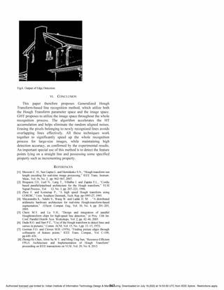
The edge detection for the corresponding input image of size
256 x 256 using the tool MODELSIM is simulated and the
output is shown in Fig. 6.
Fig.4. Input image and its Hough Transfonn-House.
lines from the Hough Transform Matrix are given below. The Fig.5. Extraction of lines-House.
846
Authorized licensed use limited to: Indian Institute of Information Technology Design & Manufacturing. Downloaded on July 19,2022 at 14:53:50 UTC from IEEE Xplore. Restrictions apply.
6.
Fig.6. Output ofEdge Detection.
VI. CONCLUSION
This paper therefore proposes Generalized Hough
Transform-based line recognition method, which utilize both
the Hough Transform parameter space and the image space.
GHT proposes to utilize the image space throughout the whole
recognition process. The algorithm accelerates the HT
accumulation and helps eliminate the random aligned noises.
Erasing the pixels belonging to newly recognized lines avoids
overlapping lines effectively. All these techniques work
together to significantly speed up the whole recognition
process for large-size images, while maintaining high
detection accuracy, as confirmed by the experimental results.
An important special use of this method is to detect the feature
points lying on a straight line and possessing some specified
property such as incrementing property.
REFERENCES
[II Messom C. H.,Sen Gupta G. and Demidenko S.N.,"Hough transform run
length encoding for real-time image processing," IEEE Trans. Instrum.
Meas., Vol. 56,No. 3, pp. 962-967,2007.
[21 Bruguera J.D., Guil N., Lang T., Villalba J. and Zapata E.L.,"Cordic
based parallel/pipelined architecture for the Hough transform," VLSI
Signal Process., Vol. 12,No.3,pp. 207-221,1996.
[
31 Zhou F. and Kornerup P., "A high speed Hough transform using
CORDIC," Univ. Southern Denmark,Tech. Rep. pp-1995-27,1995.
[41 Mayasandra K.,Salehi S.,Wang W. and Ladak H. M. ,"A distributed
arithmetic hardware architecture for real-time Hough-transform-based
segmentation," J.Electr. Comput. Eng., Vol. 30, No. 4, pp. 201-205,
2005.
[51 Chern M.Y. and Lu Y.H., "Design and integration of parallel
Houghtransform chips for high-speed line detection," in Proc. IIth Int.
Conf. Parallel Distrib. Syst. Workshops, Vol. 2,pp. 42-46,2005.
[61 Duda R.O. and Hart P.E.,"Use of the Hough transform to detect lines and
curves in pictures," Comm. ACM, Vol. 15,No. I,
pp. II-IS,1972.
[71 Gorman F.O. and Clowes M.B. (1976),"Finding picture edges through
collinearity of feature points," IEEE Trans. Comput., Vol. C-100,
pp.449-456.
[81 Zhong-Ho Chen,Alvin Su W.Y. and Ming-Ting Sun,"Resource-Efficient
FPGA Architecture and Implementation of Hough Transform "
proceeding on IEEE transactions on VLSI ,Vol. 20,No. 8,2012.
847
Authorized licensed use limited to: Indian Institute of Information Technology Design & Manufacturing. Downloaded on July 19,2022 at 14:53:50 UTC from IEEE Xplore. Restrictions apply.
View publication stats

![International Conference on Communication and Signal Processing, April 3-5, 2014, India
Implementation of Hough Transform for Image
Processing Applications
L. Chandrasekar and G. Durga
Abstract-Hough Transform (HT) can provide a significant
solution to the problems associated with line detection in an
image. Line detection is used to detect the presence of lines in an
image, at a particular orientation. The importance of line
detection is used for detecting sharp changes in image brightness.
HT is a popular technique in computer vision. The HT for line
detection replaces the original problem of detecting collinear
points in an image space by a simpler task of finding peak points
in a parameter space. The proposed method used in this paper is
to implement Generalized Hough Transform (GHT) on an image,
since in GHT any straight line in the image is represented by a
single point in the (p,9) parameter space and any part of this
straight line is transformed into the same point. It can compute
the HT of 256 x 256 test images. It can able to detect the lines
present in the image and also it can extract feature points in an
image.
Index Terms-Generalized Hough Transform, Hough
Transform, parameter space.
I. INTRODUCTION
A
UTOMATIC detection of lines in images is a classic
problem in computer vision and image processing.
Extracting target lines efficiently and accurately are necessary
requirements for real-time applications. The Hough Transform
[1] is an efficient tool for detecting straight lines in images
even in the presence of noise and missing data. HT for line
detection is a voting process where each feature points votes
for all possible lines passing through that point. These votes
are then accumulated in an accumulator array called as Hough
Space (HS). In general, by preprocessing and thresholding, the
images are converted into binary feature image with binary
pixel values. A line can able to pass through several features
points that are present in image space. Assuming we draw
lines with various angles passing through feature points, each
line can be represented as a point on (p,8) parameter space,
where p is the perpendicular distance of the straight line to the
origin and 8 is the angle between a normal to the straight line
and positive x-axis. For each instance of time a line is drawn
for a feature point, it will produce a (p,8) value can be
considered as a "vote". After preprocessing all the feature
L. Chandrasekar,P.G Scholar,ECE Department,SSN College of
Engineering,Chennai,India (e-mail: Ichandrasekarl990@gmail.com).
G. Durga,Assistant Professor,ECE Department,SSN College of
Engineering,Chennai,India (e-mail: durgag@ssn.edu.in).
978-1-4799-3358-7114/$31.00 ©2014 IEEE
843
points the (p,8) value has the largest votes will correspond to
the line which passes through the largest number of feature
points. In general there are two sets of parametric
representation used for HT, one is slope-intercept based and
other one is (p,8) based. The main difference between first
and second representation is the unbounded parameter space.
The approaches used in HT are Co-Ordinate Rotation Digital
Computer (CORDIC) algorithm and Distributed Arithmetic
(DA). In this paper, Generalized Hough Transform (GHT)
algorithm is used to detect lines in image and extracting the
feature points from the GHT matrix which are having the
maximum peak values.
The rest of this paper is organized as follows. Section II
provides a literature review of related works. Section III
describes the detailed study of Hough Transform. Section IV
describes the proposed Generalized Hough Transform. Section
V evaluates the simulation results. Finally, a conclusion is
given in Section VI.
II. LITERATURE RE VIEW
The Hough Transform using CORDIC [2] is widely used
in image processing and recognition. CORDIC is an arithmetic
technique which is used to solve the trigonometric problems
by rotating a vector in small angle until the desired angle is
achieved. The CORDIC algorithm uses adders and shifters to
easily realize the trigonometric function calculation together
with the multiplications needed in Hough Transform. Though
the pipelined CORDIC [3] structure proposed can reach a high
calculation speed, it requires more number of adders and
shifters to realize the Hough transform in real time. In order to
perform the calculation in real time, parallel structures are
needed. Such parallel structure can take long time to perform
computation. However the cost is also very high. High speed
Hough Transform is obtained by unfolding CORDIC
algorithm into a pipelined structure, this make the architecture
very complex. It takes a long time to perform the Hough
transform. The major drawbacks are it requires multiple
iteration in parameter space and the required resources are also
increased. To compute a single p (perpendicular distance of
the straight line in the image from any pixel to the origin)
value CORDIC requires the trigonometry functions such as
sine and cosine. Another drawback of CORDIC is that the
result produced is not the correct value but the correct value
with a constant "gain". The gain can be eliminated by
applying an inverse gain to the initialization vector. However
this also requires additional resources.
The Hough transform using DA is described in [4]. It
emerges as an effective choice towards the addition of
+-IEEE
Advancing Technology
for Humanity
Authorized licensed use limited to: Indian Institute of Information Technology Design & Manufacturing. Downloaded on July 19,2022 at 14:53:50 UTC from IEEE Xplore. Restrictions apply.](https://image.slidesharecdn.com/implementationofhoughtransformforimageprocessingapplications-250522215418-999eaaf3/85/Implementation_of_Hough_Transform_for_image_processing_applications-pdf-2-320.jpg)
![extraneous noise and performs line detection even when the
lines in the image contain gaps. Once all the points in an
image are transformed using this method, the Hough
parameter space can be inspected for local maxima which
indicate the orientation and the position of the straight lines in
the original image. The Hough accumulator array thus serves
as an indicator of the exact position of the straight line in the
image. The main drawbacks of DA are its high memory
requirements and computational complexity, and these impose
a limitation on the use of the transform for real-time
applications. However, the transform is computationally
expensive and the standard form is ineffective for real-time
segmentation applications.
Line detection [5] is often needed in computer vision
applications. The Hough transform processing of image data
for line detection is robust but time-consuming. With the use
of multiple processors, the processing time for Hough
transform can be much reduced. The Hough transform needs
accumulator memory to store the voting count in each
probable parameter point. It could obtain a point in the
parameter space by a single accumulation. However, all of the
pixels in the binary feature image need to go through the
computation pixel by pixel, which limits its throughput.
III. DETAILED STUDY OF HOUGH TRANSFORM
The Hough Transform is used for the detection of features
of a particular shape like lines or circles in digitalized images.
The Hough transform has long been recognized as a robust
technique for detecting multi-dimensional features in an image
and estimating their parameters. It has many applications, as
most manufactured parts contain feature boundaries, which
can be described by regular curves or straight lines. Its main
advantage is that it is tolerant of gaps in feature boundary
descriptions and is relatively unaffected by noisy image.
The purpose of the technique is to fmd imperfect instances
of objects within a certain class of shapes by a voting
procedure. This voting procedure is carried out in a parameter
space, from which object candidates are obtained as local
maxima in a accumulator space that is explicitly constructed
by the algorithm for computing the Hough transform. It
transforms between the Cartesian space and a parameter space
in which a straight line can be defmed [6]. Let's consider the
case where we have straight lines in an image. We first note
that for every point (Xi, Yi) in that image, all the straight lines
passing through that point satisfy (1) for varying values of line
slope and intercept (m, c).
Yi = mXi + C (1)
Now if we reverse our variables and look instead at the values
of (m, c) as a function of the image point co-ordinates (Xi, Yi)
then (1) becomes
(2)
Equation (2) describes a straight line on a graph of c against
m. Following the discussion above, we now can describe an
algorithm for detecting lines in images. The steps are as
follows:
1. Find all the line points in the image using any suitable line
detection scheme.
2. Quantize the (m, c) space into a two-dimensional matrix H
with appropriate quantization levels.
3. Initialize the matrix H to zero.
4. Each element of H matrix, H(mi' Ci), which is found to
correspond to an line point is incremented by 1. The result is a
histogram or a vote matrix showing the frequency of line
points corresponding to certain (m, c) values (i.e. points lying
on a common line).
5. The histogram H is thresholded where only the large valued
elements are taken. These elements correspond to lines in the
original image.
In Classical Hough Transform, the lines and curves are
defined by slope-intercept parameters and in Generalized
Hough Transform which are defined by angle-radius
parameters.
A. Classical Hough Transform
The Classical Hough Transform [7] is a standard algorithm
for line and circle detection. It can be applied to many
computer vision problems as most images contain feature
boundaries which can be described by regular curves. The
main advantage of the Hough transform technique is that it is
tolerant of gaps in feature boundary descriptions and is
relatively unaffected by image noise, unlike line detectors.
The simplest case of Hough transform is the linear
transform for detecting straight lines. In the image space, the
straight line can be described as Y = mx + C and can be
graphically plotted for each pair of image points (x, y). In the
Hough transform, a main idea is to consider the characteristics
of the straight line not as image points x or y, but in terms of
its parameters, here the slope parameter m and the intercept
parameter c. However, this method has its drawbacks. If the
line is horizontal, then m is 0, and if the line is vertical, then
m is infinite.
Since the slope of vertical line is not defined, the classical
Hough transform is not suitable for vertical lines. The
drawback of classical Hough transform is, it gives an infmite
line which is expressed by the pair of m and C values, rather
than a finite line segment with two well defmed end points.
One practical difficulty is that, the Y = mx + C form for
representing a straight line breaks down for vertical lines,
when m becomes infinite. It is impossible to detect vertical
lines in an image by this method. To overcome the above
problem, Generalized Hough Transform method is introduced.
IV. PROPOSED GENERALIZED HOUGH TRANSFORM
A. Generalized Hough Transform
The Generalized Hough Transform is the modification of
the Hough Transform using the principle of template
matching. This modification enables the Hough Transform to
be used for not only the detection of an object described with
an analytic equation (e.g. line, circle, etc.) and it can also be
used to detect an arbitrary object described with its model. The
problem of finding the object (described with a model) in an
image can be solved by fmding the model's position in the
844
Authorized licensed use limited to: Indian Institute of Information Technology Design & Manufacturing. Downloaded on July 19,2022 at 14:53:50 UTC from IEEE Xplore. Restrictions apply.](https://image.slidesharecdn.com/implementationofhoughtransformforimageprocessingapplications-250522215418-999eaaf3/85/Implementation_of_Hough_Transform_for_image_processing_applications-pdf-3-320.jpg)
![image. With the Generalized Hough Transform, the problem
of finding the model's position is transformed to a problem of
fmding the transformation's parameter that maps the model
into the image. As long as we know the value of the
transformation's parameter, the position of the model in the
image can be determined [8]. The original implementation of
the GHT uses line information to define a mapping from
orientation of a line point to a reference point of the shape.
In the case of a binary image where pixels can be either
black or white, every black pixel of the image can be a black
pixel of the desired pattern thus creating a locus of reference
points in the Hough Space. Every pixel of the image votes for
its corresponding reference points. The maximum points of the
Hough Space indicate possible reference points of the pattern
in the image. This maximum can be found by scanning the
Hough Space or by solving a relaxed set of equations, each of
them corresponding to a black pixel. In Generalized Hough
transform, the ;space is converted into p-e space. So, a
more general representation of a line will be
p = x cose + ysine (3)
The drawbacks of Classical Hough transform are overcome
by Generalized Hough transform. In GHT the (x,y) space is
converted into (p,e) parameter space. From the Fig. 1, it is
noted that p is the perpendicular distance of the straight line
from the point P(x,y) to the origin 0 and e is the angle
between a normal to the straight line and the positive x-axis
and AB is the line segment in xy-space and draw one
perpendicular line segment from the point P(x,y) to positive
x-axis, mark the meeting point as Rand OP is equal to p.
From the Fig. 1, slope of the line segment OP is tane. Since
the line segment AB is perpendicular to OP, the slope of AB is
given by (4).
Use (4) and (5) in the general form of straight line segment
AB, we get
cose p
y = - -- x + --
sine sine
and it can be written as
p = x cose + ysine
(6)
(7)
Hence the (7) is used in Generalized Hough Transform to
convert the xy-space into (p,e) parameter space. In (7) x and
y are the image co- ordinates which are kept constants, p and
e are variables. For a single pixel (single point) we can
calculate different p values by varying the values of e. Points
in an image (Points in (x,y) space) are equivalent to sinusoids
in parameter space as shown in Fig. 2 and Fig. 3 respectively.
Similarly point in parameter space is equivalent to the line in
image (i.e.,) a point in parameter space is obtained by
intersection of several sinusoids which is equivalent to the
straight lines in image.
y'
II
cose
m = - -
sine
(4) Fig.2. Representation of line in (X, y) space.
y
x
B
Fig.l. Conversion of Xy-space into (p,e) parameter space.
In Fig. 1, the line segment AB meet the y-axis at the point
Q(D,c) and from the right-angle llOPQ, the y-intercept is
given by (5)
p
c = -
sine
(5)
845
ParameterSpace (p,e) -�..,
-�I)I
- 11.11
-� III
-�'PI
.,
..
Fig.3. Representation of line in (p,e) parameter space.
Fig. 2 shows that a line is represented in (x,y) space in
which a set of pixels passing through it. In Fig. 3 the same line
is represented in (p,e) parameter space. The Algorithm for
Generalized Hough transform algorithm is given in the
following steps
Authorized licensed use limited to: Indian Institute of Information Technology Design & Manufacturing. Downloaded on July 19,2022 at 14:53:50 UTC from IEEE Xplore. Restrictions apply.](https://image.slidesharecdn.com/implementationofhoughtransformforimageprocessingapplications-250522215418-999eaaf3/85/Implementation_of_Hough_Transform_for_image_processing_applications-pdf-4-320.jpg)
![Step 1: Read the input image with size of W xH.
Step 2: By preprocessing and thresholding, convert the input
image into binary feature image.
Step 3: Calculate R = round (-J�(W----1-::-:)2::-+
----:-
(H
---
-----:
1)
""" 2·).
Step 4: Build Rho which varies from - R to R with spacing
Rho-resolution (user defined).
Step 5: Build Theta which varies from - 90 to 90 with spacing
Theta-Resolution (user defined).
Step 6: Calculate NR and NT, where NR = Number of
elements in Rho matrix and NT = Number of elements in
Theta matrix.
Step 7: Build a Hough Transform Matrix (HTM) with zero
elements of size NR xNT
Step 8: Find the co-ordinates (x, y) of all feature pixels and
the number of feature pixels (P) in binary feature image.
Step 9: Create a accumulator (ace) with zero elements of
P xNT.
Step 10: Calculate all the values of Sand C, where
S = [0 to H - 1] xsin(Theta)
C = [0 to W - 1] xcos(Theta)
Step 11: Find C(x) and S(y) such that C(x) is the value of C
present only for the x co-ordinates and S(y) is the value of S
present only in y co-ordinates.
Step 12: Now calculate ace = round [C(x) + S(y)], ace is
nothing but the perpendicular distances (p values) for the
feature pixels in the binary image.
Step 13: Comparing ace and Rho, calculate a and b, where a
indicates the row in which the element present in ace and b
indicates the column in which the element present in Rho
should be as same as that of the element in acematrix.
Step 14:Increment the HTM by HT
M(a,b) = HT
M(a,b) + 1.
Step 15: Plot the HTM along with Rho and Theta. Hence the
lines are detected.
B. Feature Extraction
The algorithm uses an optimal line detector based on a set
of criteria which include finding the most lines by minimizing
the error rate, marking lines as closely as possible to the actual
lines to maximize localization, and marking lines only once
when a single line exists for minimal response. The Algorithm
for extracting lines from Hough Transform Matrix is given in
the following steps
Step 1: Find the number of peaks in HTM.
Step 2: Find the row(p) and column(q) of the first peak from
HTM.
Step 3: Map the p with Rho and find the p value and similarly
map the q with Thetaand find the () value.
Step 4: Find the co-ordinates of the pixels which give
corresponding p and ().
Step 5: Repeat Step 2, Step 3 and Step 4 for all peaks.
Step 6: Plot the co-ordinates of the pixels on the binary feature
image.
V. SIMULATION RESULTS
The tool used for simulation is MATrix LABoratory
(MATLAB). The results for line detection and extraction of
input image is the house which is in the size of 256 x 256, the
lines in the input image are detected in its corresponding
Hough Transform of input image as shown in Fig. 4. The lines
in the image are detected as a number of points in the Rho and
Theta parameter space. The votes for collinear points are
consolidated in the Hough Transform Matrix and then plotted
in (p,()) parameter space.
In extraction process, the lines are retrieved from the
image. The lines are extracted from the HTM which is
generated from the Algorithm of Generalized Hough
Transform. The input image is as same as shown in Fig. 4. The
extracted lines for the input image house are shown in Fig. 5.
The threshold value is given in order to find the number of
peaks in HTM. The peak which has the highest accumulated
votes is extracted first. The co-ordinates of the peak are
determined and then its drawn on the binary feature image.
The number of collinear pixels is detected on basis of the peak
value which has the largest accumulated votes from the HTM.
The edge detection for the corresponding input image of size
256 x 256 using the tool MODELSIM is simulated and the
output is shown in Fig. 6.
Fig.4. Input image and its Hough Transfonn-House.
lines from the Hough Transform Matrix are given below. The Fig.5. Extraction of lines-House.
846
Authorized licensed use limited to: Indian Institute of Information Technology Design & Manufacturing. Downloaded on July 19,2022 at 14:53:50 UTC from IEEE Xplore. Restrictions apply.](https://image.slidesharecdn.com/implementationofhoughtransformforimageprocessingapplications-250522215418-999eaaf3/85/Implementation_of_Hough_Transform_for_image_processing_applications-pdf-5-320.jpg)