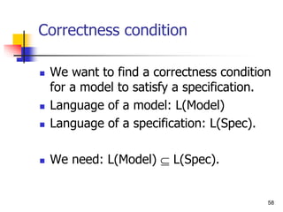
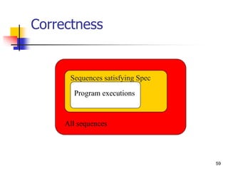
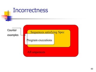
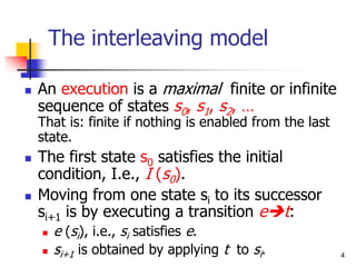
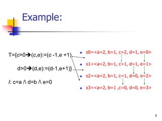
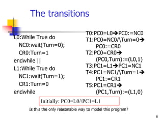
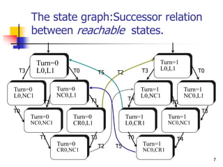
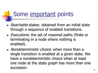
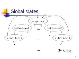
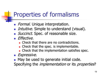
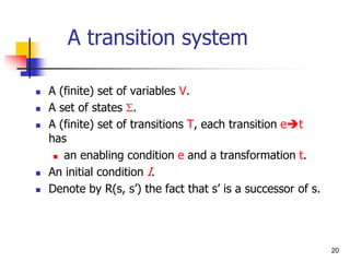
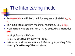
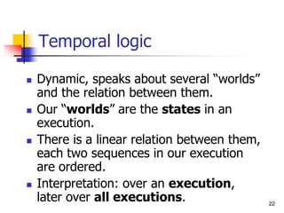
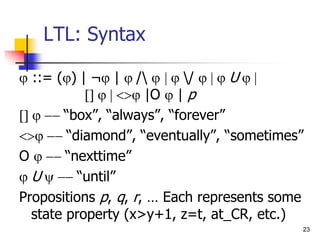
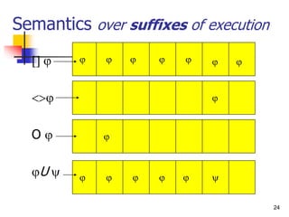
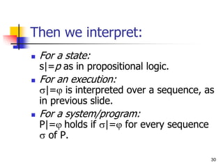
This document discusses transition systems and their modeling using temporal logic. It begins by defining a transition system as consisting of variables, states, transitions between states, and an initial condition. An execution is defined as a sequence of states. Temporal logic is then introduced as a way to specify properties of transitions systems over executions. The semantics of temporal logic operators such as "always" ([]), "eventually" (<>), and "until" (U) are defined over suffixes of executions. Various properties and relationships between temporal logic formulas are discussed. Finally, satisfaction of formulas by single sequences and by transition systems is defined.


![25
Can discard some operators
Instead of <>p, write true U p.
Instead of []p, we can write ¬(<>¬p),
or ¬(true U ¬p).
Because []p=¬¬[]p.
¬[]p means it is not true that p holds
forever, or at some point ¬p holds or
<>¬p.](https://image.slidesharecdn.com/lecture10fm-240110045843-1b41df83/85/lecture-10-formal-methods-in-software-enginnering-pptx-25-320.jpg)
![26
Combinations
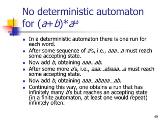
[]<>p “p will happen infinitely often”
<>[]p “p will happen from some point
forever”.
([]<>p) ([]<>q) “If p happens
infinitely often, then q also happens
infinitely often”.](https://image.slidesharecdn.com/lecture10fm-240110045843-1b41df83/85/lecture-10-formal-methods-in-software-enginnering-pptx-26-320.jpg)
=([])/([])
But <>(/)(<>)/(<>)
<>(/)=(<>)/(<>)
But [](/)([])/([])
](https://image.slidesharecdn.com/lecture10fm-240110045843-1b41df83/85/lecture-10-formal-methods-in-software-enginnering-pptx-27-320.jpg)
![28
What about
([]<>)/([]<>)=[]<>(/)?
([]<>)/([]<>)=[]<>(/)?
(<>[])/(<>[])=<>[](/)?
(<>[])/(<>[])=<>[](/)?
No, just
Yes!!!
Yes!!!
No, just ](https://image.slidesharecdn.com/lecture10fm-240110045843-1b41df83/85/lecture-10-formal-methods-in-software-enginnering-pptx-28-320.jpg)
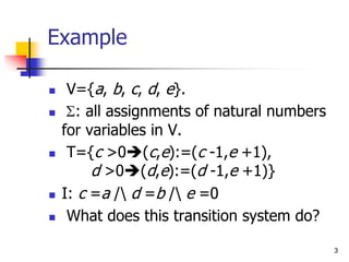
![29
Formal semantic definition
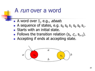
Let be a sequence s0 s1 s2 …
Let i be a suffix of : si si+1 si+2 … (0 = )
i |= p, where p a proposition, if si|=p.
i |= / if i |= and i |= .
i |= / if i |= or i |= .
i |= ¬ if it is not the case that i |= .
i |= <> if for some ji, j |= .
i |= [] if for each ji, j |= .
i |= U if for some ji, j|=.
and for each ik<j, k |=.](https://image.slidesharecdn.com/lecture10fm-240110045843-1b41df83/85/lecture-10-formal-methods-in-software-enginnering-pptx-29-320.jpg)
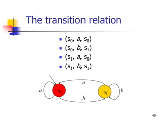
![32
LTL satisfaction by a single
sequence
malfunction
s1 s3
s2
pull
release
release
extended extended
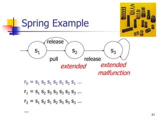
r2 = s1 s2 s1 s2 s3 s3 s3 …
r2 |= extended ??
r2 |= O extended ??
r2 |= O O extended ??
r2 |= <> extended ??
r2 |= [] extended ??
r2 |= <>[] extended ??
r2 |= ¬ <>[] extended ??
r2 |= (¬extended) U malfunction ??
r2 |= [](¬extended->O extended) ??](https://image.slidesharecdn.com/lecture10fm-240110045843-1b41df83/85/lecture-10-formal-methods-in-software-enginnering-pptx-32-320.jpg)
![33
LTL satisfaction by a system
malfunction
s1 s3
s2
pull
release
release
extended extended
P |= extended ??
P |= O extended ??
P |= O O extended ??
P |= <> extended ??
P|= [] extended ??
P |= <>[] extended ??
P |= ¬ <>[] extended ??
P |= (¬extended) U malfunction ??
P |= [](¬extended->O extended) ??](https://image.slidesharecdn.com/lecture10fm-240110045843-1b41df83/85/lecture-10-formal-methods-in-software-enginnering-pptx-33-320.jpg)
![34
More specifications
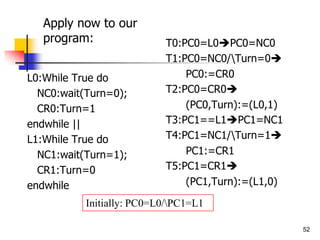
[] (PC0=NC0 <> PC0=CR0)
[] (PC0=NC0 U Turn=0)
Try at home:
- The processes alternate in entering
their critical sections.
- Each process enters its critical section
infinitely often.](https://image.slidesharecdn.com/lecture10fm-240110045843-1b41df83/85/lecture-10-formal-methods-in-software-enginnering-pptx-34-320.jpg)
![35
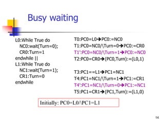
Proof system
¬<>p<-->[]¬p
[](pq)([]p[]q)
[]p(p/O[]p)
O¬p<-->¬Op
[](pOp)(p[]p)
(pUq)<-->(q/(p/O(pUq)))
(pUq)<>q
+ propositional logic
axiomatization.
+ proof rule:
_p_
[]p](https://image.slidesharecdn.com/lecture10fm-240110045843-1b41df83/85/lecture-10-formal-methods-in-software-enginnering-pptx-35-320.jpg)
/¬(ye/re)/¬(re/gr)/(gr/ye/re))
Correct change of color:
[]((grU ye)/(yeU re)/(reU gr))](https://image.slidesharecdn.com/lecture10fm-240110045843-1b41df83/85/lecture-10-formal-methods-in-software-enginnering-pptx-36-320.jpg)
 U ye)/(ye U (gr/re)))
Correct specification:
[]( (gr(gr U (ye / ( ye U re ))))
/(re(re U (ye / ( ye U gr ))))
/(ye(ye U (gr / re))))
Needed only when we
can start with yellow](https://image.slidesharecdn.com/lecture10fm-240110045843-1b41df83/85/lecture-10-formal-methods-in-software-enginnering-pptx-37-320.jpg)

Termination: init/<>finish
Total correctness: init/<>(finish/ )
Invariant: init/[]](https://image.slidesharecdn.com/lecture10fm-240110045843-1b41df83/85/lecture-10-formal-methods-in-software-enginnering-pptx-38-320.jpg)
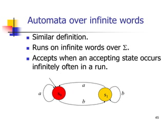
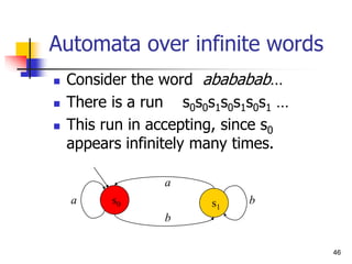
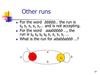
![50
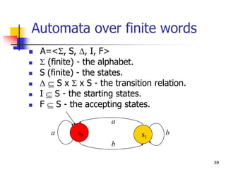
Specification using Automata
Let each letter correspond to some propositional
property.
Example: a -- P0 enters critical section,
b -- P0 does not enter section.
[]<>PC0=CR0
a
a
b
b
s0 s1](https://image.slidesharecdn.com/lecture10fm-240110045843-1b41df83/85/lecture-10-formal-methods-in-software-enginnering-pptx-50-320.jpg)
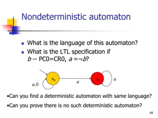
![51
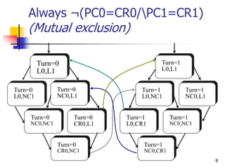
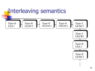
Mutual Exclusion
a -- PC0=CR0/PC1=CR1
b -- ¬(PC0=CR0/PC1=CR1)
c -- true
[]¬(PC0=CR0/PC1=CR1)
b a c
s0 s1](https://image.slidesharecdn.com/lecture10fm-240110045843-1b41df83/85/lecture-10-formal-methods-in-software-enginnering-pptx-51-320.jpg)
![54
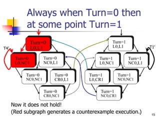
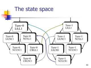
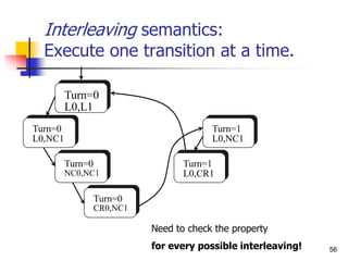
[]¬(PC0=CR0/PC1=CR1)
(Mutual exclusion)
Turn=0
L0,L1
Turn=0
L0,NC1
Turn=0
NC0,L1
Turn=0
CR0,NC1
Turn=0
NC0,NC1
Turn=0
CR0,L1
Turn=1
L0,CR1
Turn=1
NC0,CR1
Turn=1
L0,NC1
Turn=1
NC0,NC1
Turn=1
NC0,L1
Turn=1
L0,L1](https://image.slidesharecdn.com/lecture10fm-240110045843-1b41df83/85/lecture-10-formal-methods-in-software-enginnering-pptx-54-320.jpg)

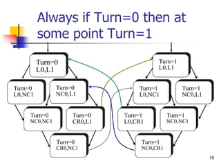
Turn=0
L0,L1
Turn=0
L0,NC1
Turn=0
NC0,L1
Turn=0
CR0,NC1
Turn=0
NC0,NC1
Turn=0
CR0,L1
Turn=1
L0,CR1
Turn=1
NC0,CR1
Turn=1
L0,NC1
Turn=1
NC0,NC1
Turn=1
NC0,L1
Turn=1
L0,L1](https://image.slidesharecdn.com/lecture10fm-240110045843-1b41df83/85/lecture-10-formal-methods-in-software-enginnering-pptx-55-320.jpg)

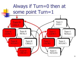
Turn=0
L0,L1
Turn=0
L0,NC1
Turn=0
NC0,L1
Turn=0
CR0,NC1
Turn=0
NC0,NC1
Turn=0
CR0,L1
Turn=1
L0,CR1
Turn=1
NC0,CR1
Turn=1
L0,NC1
Turn=1
NC0,NC1
Turn=1
NC0,L1
Turn=1
L0,L1](https://image.slidesharecdn.com/lecture10fm-240110045843-1b41df83/85/lecture-10-formal-methods-in-software-enginnering-pptx-57-320.jpg)