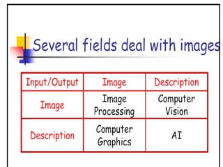
This document provides information about an image processing course. The key details are:
- The course number is CSC 447 and is taught over 3 lecture hours and 2 lab hours. It is worth 65 marks and has a 3 hour exam.
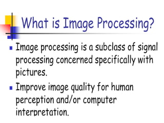
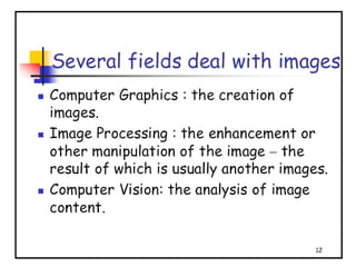
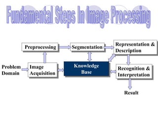
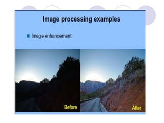
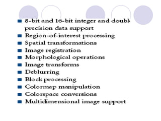
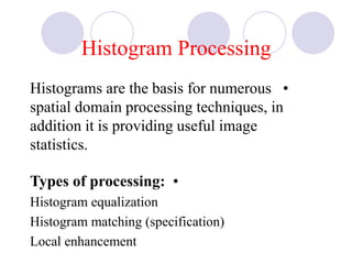
- The course covers topics like image processing applications, enhancement techniques, restoration, segmentation, and scene analysis. It also covers specific techniques like using neural networks and parallel algorithms for image processing.
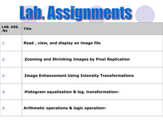
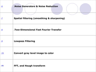
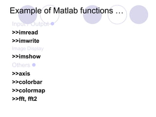
- The textbook for the course is "Digital Image Processing Using Matlab" by Rafael Gonzalez and Richard Woods. There are 11 lab assignments focused on topics like image display, filtering, transforms, and color conversion using Matlab.
- The course is taught by


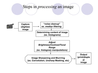
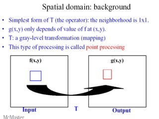
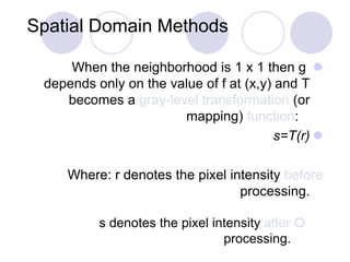
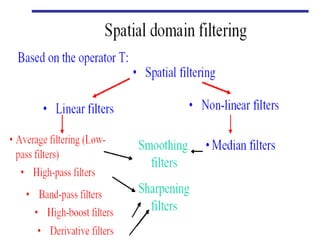
![Spatial Domain Methods
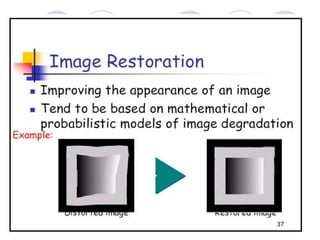
Procedures that operate directly on the
aggregate of pixels composing an
image
A neighborhood about (x,y) is defined
by using a square (or rectangular)
subimage area centered at (x,y).
)],([),( yxfTyxg ](https://image.slidesharecdn.com/imageprocessing-1-lectures-200214110926/85/Image-processing-1-lectures-84-320.jpg)
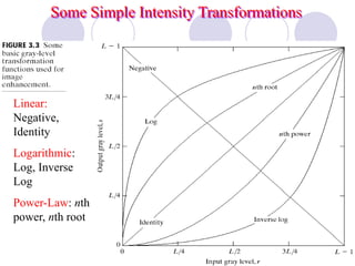
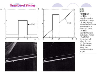
![1-Image Negatives
Are obtained by using the
transformation function s=T(r).
[0,L-1] the range of gray levels
S= L-1-r](https://image.slidesharecdn.com/imageprocessing-1-lectures-200214110926/85/Image-processing-1-lectures-89-320.jpg)
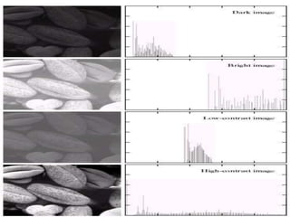
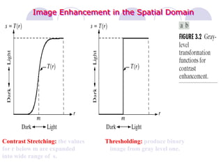
![Histogram stretching:
For an image f(x,y) with gray level r at x,y this value can be transformed
to another gray level value s in the new image g(x,y), using the following
equ.:
g(x,y) = [(r- rmin) / ( rmax- rmin)] * [Max-Min] +Min
Where: rmax is the largest gray level in the image f(x,y).
rmin is the smallest gray level in the image f(x,y).
Max, Min correspond to the maximum and minimum
gray level values possible for the image g(x,y), (0-255).
Histogram shrinking :
g(x,y) = [( Max - Min ) / (rmax-rmin)] * [r – rmin] + Min
Where: Max, Min correspond to the maximum and minimum
desired gray level in the compressed (shrink) histogram.](https://image.slidesharecdn.com/imageprocessing-1-lectures-200214110926/85/Image-processing-1-lectures-108-320.jpg)
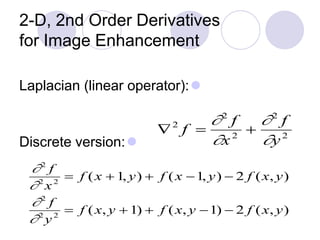
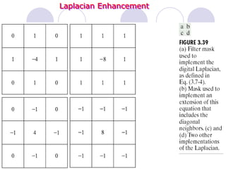
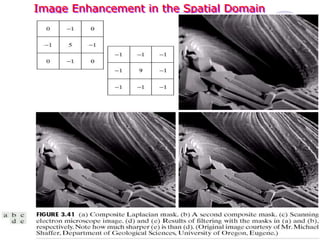
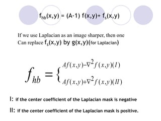
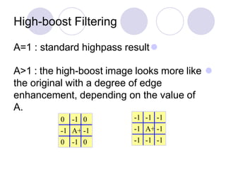
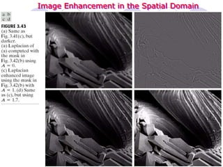
![Laplacian
Digital implementation:
Two definitions of Laplacian: one is the negative of the other
Accordingly, to recover background features:
: if the center coefficient of the Laplacian mask is negative
II: if the center coefficient of the Laplacian mask is positive.
2
f [f (x +1,y)+ f (x1,y)+ f (x,y +1)+ f (x,y1)]4 f (x,y)
g(x,y) { f ( x,y)+2 f ( x,y)( II )
f ( x,y)2 f ( x,y)( I )](https://image.slidesharecdn.com/imageprocessing-1-lectures-200214110926/85/Image-processing-1-lectures-161-320.jpg)
![Simplification
Filter and recover original part in one step:
g(x,y) f(x,y)[f(x+1,y)+ f(x1,y)+ f(x,y+1)+ f(x,y1)]+4f(x,y)
g(x,y) 5f (x,y)[ f (x +1,y)+ f (x 1,y)+ f (x,y +1)+ f (x,y 1)]](https://image.slidesharecdn.com/imageprocessing-1-lectures-200214110926/85/Image-processing-1-lectures-163-320.jpg)