This document discusses dimensionality reduction techniques. It explains that dimensionality reduction can be used to simplify complex high-dimensional data by summarizing it with a lower dimensional real-valued vector while minimizing information loss. Principal component analysis (PCA) is described as a technique that finds the directions along which the variance of the data is maximized to reduce dimensionality. Examples of applying PCA to compress image data from high to lower dimensions are provided.

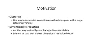
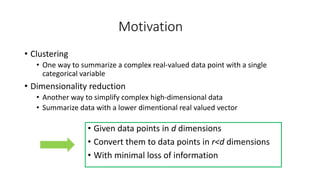
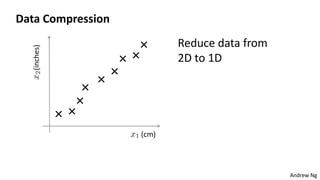
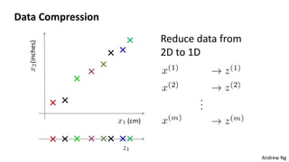
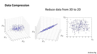
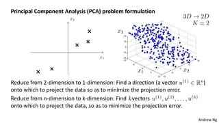
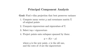
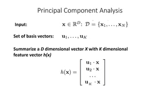
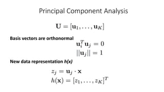
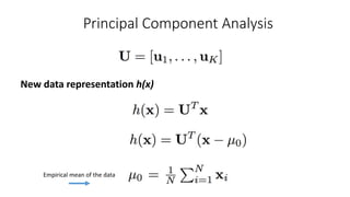
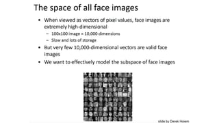
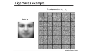
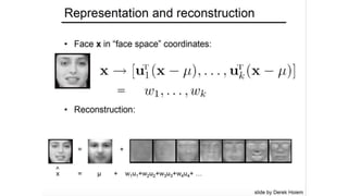
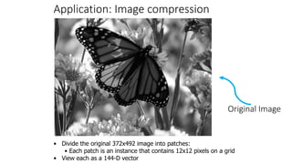
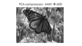
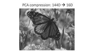
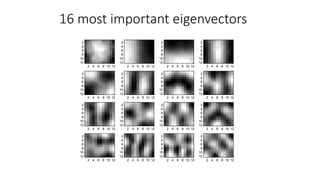
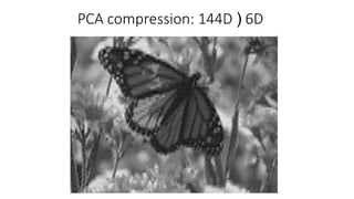
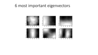
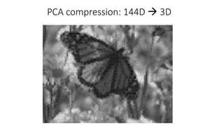
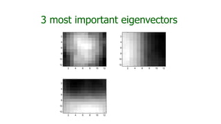
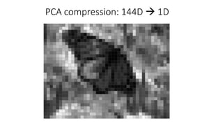
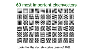
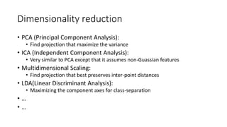
1. Dimensionality Reduction
Fereshteh Sadeghi
CSEP 546

2. Motivation
• Clustering
• One way to summarize a complex real-valued data point with a single
categorical variable
• Dimensionality reduction
• Another way to simplify complex high-dimensional data
• Summarize data with a lower dimensional real valued vector

3. Motivation
• Clustering
• One way to summarize a complex real-valued data point with a single
categorical variable
• Dimensionality reduction
• Another way to simplify complex high-dimensional data
• Summarize data with a lower dimentional real valued vector
• Given data points in d dimensions
• Convert them to data points in r<d dimensions
• With minimal loss of information

4. Data Compression
(inches)
(cm)
Reduce data from
2D to 1D
Andrew Ng

5. Data Compression
Reduce data from
2D to 1D
(inches)
(cm)
Andrew Ng

6. Data Compression
Reduce data from 3D to 2D
Andrew Ng

7. Principal Component Analysis (PCA) problem formulation
Reduce from 2-dimension to 1-dimension: Find a direction (a vector )
onto which to project the data so as to minimize the projection error.
Reduce from n-dimension to k-dimension: Find vectors
onto which to project the data, so as to minimize the projection error.
Andrew Ng

9. Covariance
• Variance and Covariance:
• Measure of the “spread” of a set of points around their center of mass(mean)
• Variance:
• Measure of the deviation from the mean for points in one dimension
• Covariance:
• Measure of how much each of the dimensions vary from the mean with
respect to each other
• Covariance is measured between two dimensions
• Covariance sees if there is a relation between two dimensions
• Covariance between one dimension is the variance

10. Positive: Both dimensions increase or decrease together Negative: While one increase the other decrease

11. Covariance
• Used to find relationships between dimensions in high dimensional
data sets
The Sample mean

12. Eigenvector and Eigenvalue
Ax = λx
A: Square Matirx
λ: Eigenvector or characteristic vector
X: Eigenvalue or characteristic value
• The zero vector can not be an eigenvector
• The value zero can be eigenvalue

13. Eigenvector and Eigenvalue
Ax = λx
A: Square Matirx
λ: Eigenvector or characteristic vector
X: Eigenvalue or characteristic value
Example

14. Eigenvector and Eigenvalue
Ax - λx = 0
(A – λI)x = 0
B = A – λI
Bx = 0
x = B-10 = 0
If we define a new matrix B:
If B has an inverse:
BUT! an eigenvector
cannot be zero!!
x will be an eigenvector of A if and only if B does
not have an inverse, or equivalently det(B)=0 :
det(A – λI) = 0
Ax = λx

15. Example 1: Find the eigenvalues of
two eigenvalues: 1,  2
Note: The roots of the characteristic equation can be repeated. That is, λ1 = λ2 =…= λk.
If that happens, the eigenvalue is said to be of multiplicity k.
Example 2: Find the eigenvalues of
λ = 2 is an eigenvector of multiplicity 3.









5
1
12
2
A
)
2
)(
1
(
2
3
12
)
5
)(
2
(
5
1
12
2
2























 A
I











2
0
0
0
2
0
0
1
2
A
0
)
2
(
2
0
0
0
2
0
0
1
2
3








 



 A
I
Eigenvector and Eigenvalue

16. Principal Component Analysis
Input:
Summarize a D dimensional vector X with K dimensional
feature vector h(x)
Set of basis vectors:

17. Principal Component Analysis
Basis vectors are orthonormal
New data representation h(x)

18. Principal Component Analysis
New data representation h(x)
Empirical mean of the data

23. • The top three principal components of SIFT descriptors from a set of images are computed
• Map these principal components to the principal components of the RGB space
• pixels with similar colors share similar structures
SIFT feature visualization

24. Original Image
• Divide the original 372x492 image into patches:
• Each patch is an instance that contains 12x12 pixels on a grid
• View each as a 144-D vector
Application: Image compression

25. PCA compression: 144D  60D

26. PCA compression: 144D  16D

27. 16 most important eigenvectors
2 4 6 8 10 12
2
4
6
8
10
12
2 4 6 8 10 12
2
4
6
8
10
12
2 4 6 8 10 12
2
4
6
8
10
12
2 4 6 8 10 12
2
4
6
8
10
12
2 4 6 8 10 12
2
4
6
8
10
12
2 4 6 8 10 12
2
4
6
8
10
12
2 4 6 8 10 12
2
4
6
8
10
12
2 4 6 8 10 12
2
4
6
8
10
12
2 4 6 8 10 12
2
4
6
8
10
12
2 4 6 8 10 12
2
4
6
8
10
12
2 4 6 8 10 12
2
4
6
8
10
12
2 4 6 8 10 12
2
4
6
8
10
12
2 4 6 8 10 12
2
4
6
8
10
12
2 4 6 8 10 12
2
4
6
8
10
12
2 4 6 8 10 12
2
4
6
8
10
12
2 4 6 8 10 12
2
4
6
8
10
12

28. PCA compression: 144D ) 6D

29. 2 4 6 8 10 12
2
4
6
8
10
12
2 4 6 8 10 12
2
4
6
8
10
12
2 4 6 8 10 12
2
4
6
8
10
12
2 4 6 8 10 12
2
4
6
8
10
12
2 4 6 8 10 12
2
4
6
8
10
12
2 4 6 8 10 12
2
4
6
8
10
12
6 most important eigenvectors

30. PCA compression: 144D  3D

31. 2 4 6 8 10 12
2
4
6
8
10
12
2 4 6 8 10 12
2
4
6
8
10
12
2 4 6 8 10 12
2
4
6
8
10
12
3 most important eigenvectors

32. PCA compression: 144D  1D

33. 60 most important eigenvectors
Looks like the discrete cosine bases of JPG!...

34. 2D Discrete Cosine Basis
http://en.wikipedia.org/wiki/Discrete_cosine_transform

35. Dimensionality reduction
• PCA (Principal Component Analysis):
• Find projection that maximize the variance
• ICA (Independent Component Analysis):
• Very similar to PCA except that it assumes non-Guassian features
• Multidimensional Scaling:
• Find projection that best preserves inter-point distances
• LDA(Linear Discriminant Analysis):
• Maximizing the component axes for class-separation
• …
• …