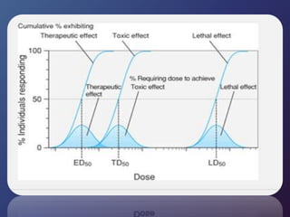
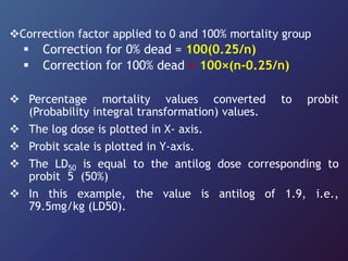
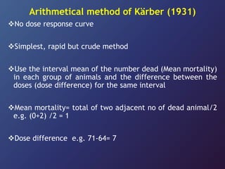
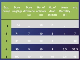
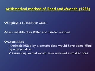
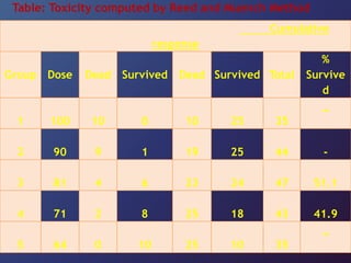
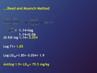
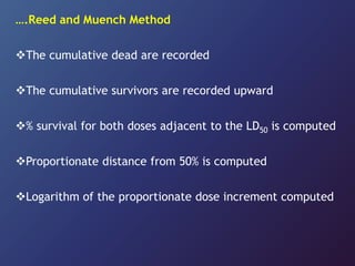
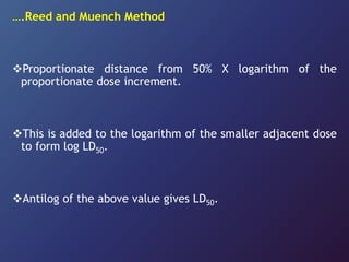
Methods to calculate
LD50 and ED50
Dr. Karabi Adak
MBBS, Md
Dose–Response Relationships
The pharmacodynamics of a drug can be quantified by
the relationship between the dose (concentration) of
the drug and the organism's (patient's) response to that
drug.
2 major types of dose–response relationships—graded
and quantal:
Graded dose–response relationships describe the
effect of various doses of a drug on an individual.
Quantal dose–response relationships show the effect
of various doses of a drug on a population of individuals.
Graded dose–response relationships
……Graded dose–response relationships
Two important parameters—potency and efficacy
The potency (EC50) of a drug is the concentration at which
the drug elicits 50% of its maximal response.
The efficacy (Emax) is the maximal response produced by the
drug.
No inter-individual variation.
Quantal Dose–Response Relationships
Plots the fraction of the population that responds to a given
dose of drug as a function of the drug dose.
The response is all-or-none.
Differences in biological response among individuals - the
effects of a drug are seen over a range of doses.
Flat curve denotes a broad range of sensitivity, a steep one
denotes a very narrow range
…….Quantal Dose–Response Relationships
Types of responses:
Median effective dose (ED50): dose at which 50% of
subjects/animals exhibit a therapeutic response to a drug.
Median toxic dose (TD50): dose at which 50% of subjects
experience a toxic response.
Median lethal dose (LD50): dose at which is lethal to 50% of
subjects.
…….Quantal Dose–Response Relationships
Values are different for each route of administration.
Both LD50 and ED50 values are important for knowing the
safety of a drug.
The ratio between LD50 and ED50 (LD50/ED50) represents
therapeutic index(TI).
Greater the TI, safer is the drug and vice-versa.
…….Quantal Dose–Response Relationships
The TI of most of the drugs which have low margin of
safety is generally close to unity.
ED99 dose that is effective in 99% of the animals of the
group.
LD10 dose that is lethal to 10% of the animals of the group.
LD50 and ED50 are mainly determined in acute toxicity
studies.
Acute Toxicity Studies
Acute toxicity refers to those adverse effects occurring
following oral administration of a single dose of a
substance, or multiple doses within 24 hr.
Aims at establishing the therapeutic index (TI)
Several species of animals are used to determine LD50
(due to species variation)
A drug effect seen both in the rat and dog probably
involves a common physiological mechanism that is
likely to be present in the human, whereas an effect
seen only in one of the two species indicate that the
same is peculiar to that species, and is less likely to be
present in the third species.
……..Acute Toxicity Studies
In practice, it is considered sufficiently adequate if LD50
with confidence limits is established on one common
laboratory species, mice or rats by the standard method.
It is unwise to use a homogenous strains (inbred strains) in
toxicity study, and the aim should be to discover new and
unexpected effects of a drug in animals of wider variability
like random bred animals.
LD50 dose, thus found is then given to guinea pigs, rabbits,
cats or dogs on the basis of their weight or surface areas.
Requirements of a toxicity study
 Should follow GLP
 Studies should be performed by well trained and
qualified staff.
 Instruments should be calibrated and standardized
properly.
 SOPs should be followed.
Acute Toxicity Test Design
First performed in mice fasted overnight (18hours)
Two rodents species(mice and rats); in each group at least 5
animals of either sex.
Route of administration-
• Same as intended for humans.
• At least one more route should be used in one of the species
to ensure systemic absorption of the drug.
• LD50 values increase with the following sequences of
routes: intravenous, intraperitoneal, subcutaneous and oral.
……Acute Toxicity Test Design
Doses-
At least three graded dose. A limit of 2g/kg (or 10 times
the normal dose that is intended in humans, whichever is
higher) is recommended for oral dosing.
Treatment- given in a single bolus or several doses or by
continuous infusion within 24 hr.
In rodents, the volume should not normally exceed
1ml/100g of body weight; however in the case of aqueous
solutions, 2 ml/100g body weight can be considered.
……Acute Toxicity Test Design
Observations-
Animals should be observed for 14 days after the drug
administration, and minimum lethal dose (MLD) and
maximum tolerated dose (MTD) and LD50 should be
established. Other features to be observed are-
Signs of intoxication
Effect on body weight
Gross pathological changes
……Acute Toxicity Test Design
Alternative method…..
Each dose given to one animal only
LD50 estimated from mean of the logarithms of the smallest
effective dose and the largest ineffective dose.
Up and down’ or ‘staircase’ method
First described by Dixon and Mood.
2 mice injected with a particular dose, eg: 175mg/kg
………Up and down’ or ‘staircase’ method
Observe for 48 hours
Dose tolerated- increase by a factor of 3.2
Dose lethal- decrease by a factor of 3.2
Maximum nonlethal dose and minimum lethal dose are thus
determined by using only about 10 mice
Economical in animal but not in time
Methods for calculating ED50
 Dixon & Massey’s method
 Reed & Muench method
 Probit method of Gaddum & Bliss
 Wilson & Worcester method
 Knudson & Curtis method
 Thompson method
 Kärber's method
Kärber's method
Based on the “S” shaped dose-response curve
The drug dosage are arranged by geometric progression
growth.
60 mice weighed, divided into 6 groups randomly, 10 mice
per group. Average weight of each group should be roughly
equal.
Geometric proportion diluents made according to the
calculated dosages.
Mice observed for 30-50 minutes after administration.
Mice showing response counted.
Positive reaction rate of each group calculated.
Table filled with the results.
…..Kärber'smethod
……Kärber's method
• ED50 calculated by the formula:
• Where, Xk=logarithm of the maximum dosage.
• i=logarithm of the ratio of the adjacent doses.
• is the sum of the positive rate of each group. P1,P2,P3,……
is the positive rate of each group.
Methods for calculating LD50
Lichtfield and Wilcoxon (1949) - Graphical method
L.C Miller and Tainter (1944) – Logarithmic probit graph
paper method
De Beer (1945) – Graphical method
Reed and Muench (1938) – Arithmetical method
Kärber (1931) – Arithmetical method
Lorke’s Method
Graphical calculation of Lichtfield and
Wilcoxon(1949)
Permits rapid estimation of LD50, slope of a dose-
percent effect curve, and the confidence limits of
both parameters for 19/20 probability using the
experimental data in their original form.
Graphical calculation of L.C Miller and Tainter
(1944)
Most commonly used method
Acurate and simple
Percentage mortality noted in the groups of animals
% 0 1 2 3 4 5 6 7 8 9
0 - 2.67 2.95 3.12 3.25 3.36 3.45 3.52 3.59 3.66
10 3.72 3.77 3.82 3.87 3.92 3.96 4.01 4.05 4.08 4.12
20 4.16 4.19 4.23 4.26 4.29 4.33 4.36 4.39 4.42 4.45
30 4.48 4.50 4.53 4.56 4.59 4.61 4.64 4.67 4.69 4.72
40 4.75 4.77 4.80 4.82 4.85 4.87 4.90 4.92 4.95 4.97
50 5.00 5.03 5.05 5.08 5.10 5.13 5.15 5.18 5.20 5.23
60 5.25 5.28 5.31 5.33 5.36 5.39 5.41 5.44 5.47 5.50
70 5.5
2
5.5
5
5.58 5.6
1
5.6
4
5.67 5.7
1
5.74 5.77 5.81
80 5.8
4
5.8
8
5.92 5.9
5
5.9
9
6.04 6.0
8
6.13 6.18 6.23
90 6.28 6.34 6.41 6.48 6.55 6.64 6.75 6.88 7.05 7.33
Group Dose
(mg/kg)
Log
dose
Dead/
Total
Dead
%
Corrected
%
Probit
1 64 1.81 0/10 0 2.5 3.04
2 71 1.85 2/10 20 20 4.16
3 81 1.91 4/10 40 40 4.75
4 90 1.95 9/10 90 90 6.28
5 100 2.00 10/10 100 97.5 6.96
Table: Results of acute toxicity study in mice
PROBIT
LOG DOSE
3
4
5
6
7
1.8 1.9 2.0
Correction factor applied to 0 and 100% mortality group
 Correction for 0% dead = 100(0.25/n)
 Correction for 100% dead = 100×(n-0.25/n)
 Percentage mortality values converted to probit
(Probability integral transformation) values.
 The log dose is plotted in X- axis.
 Probit scale is plotted in Y-axis.
 The LD50 is equal to the antilog dose corresponding to
probit 5 (50%)
 In this example, the value is antilog of 1.9, i.e.,
79.5mg/kg (LD50).
Arithmetical method of Kärber (1931)
No dose response curve
Simplest, rapid but crude method
Use the interval mean of the number dead (Mean mortality)
in each group of animals and the difference between the
doses (dose difference) for the same interval
Mean mortality= total of two adjacent no of dead animal/2
e.g. (0+2) /2 = 1
Dose difference e.g. 71-64= 7
…..Arithmetical method of Kärber
Product of the interval mean and the dose difference is
obtained (a×b) e.g 7×1=7
The product is summed up i.e., Ʃ (a×b) = 190.5
Now dividing the value by no of animals in each group =
190.5/10 = 19.05
Finally this value is subtracted from the minimum dose
which produces the 100% mortality, i.e. 100 mg/kg
So, LD50 = 100-(190.5/10) = 81 mg/kg (approx)
Exp.
Group
Dose
(mg/kg)
Dose
differene
(a)
No. of
animals
(n)
No.of
dead
animals
Mean
Mortality
(b)
a×b
1 64 _ 10 0 - -
2 71 7 10 2 1 7
3 81 10 10 4 3 30
4 90 9 10 9 6.5 58.5
5 100 10 10 10 9.5 95
Arithmetical method of Reed and Muench (1938)
Employs a cumulative value.
Less reliable than Miller and Tainter method.
Assumption:
Animals killed by a certain dose would have been killed
by a larger dose
A surviving animal would have survived a smaller dose
Table: Toxicity computed by Reed and Muench Method
Cumulative
response
Group Dose Dead Survived Dead Survived Total
%
Survive
d
1 100 10 0 10 25 35
_
2 90 9 1 19 25 44 -
3 81 4 6 23 24 47 51.1
4 71 2 8 25 18 43 41.9
5 64 0 10 25 10 35
_
(0.9)X log 1.14= 0.054
Log 71= 1.85
Log LD50=1.85+ 0.054= 1.9
Antilog 1.9= LD50= 79.5 mg/kg
1.14=log
1.14=0.06
=
….Reed and Muench Method
The cumulative dead are recorded
The cumulative survivors are recorded upward
% survival for both doses adjacent to the LD50 is computed
Proportionate distance from 50% is computed
Logarithm of the proportionate dose increment computed
….Reed and Muench Method
Proportionate distance from 50% X logarithm of the
proportionate dose increment.
This is added to the logarithm of the smaller adjacent dose
to form log LD50.
Antilog of the above value gives LD50.
Lorke’s Method
Phase 1:
Three-groups of three mice each.
One dose to each group i.p.
Monitored for 24 h for mortality and general behaviour.
Phase 2:
3–4 groups of one mouse each given doses i.p. based on the
findings of phase 1
Monitored for 24 h.
The geographic mean of the least dose that killed mice and
the highest dose that did not kill mice was taken as the
median lethal dose.
Conclusion
For many reasons TI is not a useful guide to safety
of a drug in clinical use:
LD50 based on animal toxicity data, may not
reflect toxicity in the therapeutic setting ,where
unwanted effects are rarely common but not
death.
LD50 takes no account of idiosyncratic reactions.
ED50 not definable, depends on what measures of
effectiveness is used.

LD50 and ED50.pptx

  • 1.
    Methods to calculate LD50and ED50 Dr. Karabi Adak MBBS, Md
  • 2.
    Dose–Response Relationships The pharmacodynamicsof a drug can be quantified by the relationship between the dose (concentration) of the drug and the organism's (patient's) response to that drug. 2 major types of dose–response relationships—graded and quantal: Graded dose–response relationships describe the effect of various doses of a drug on an individual. Quantal dose–response relationships show the effect of various doses of a drug on a population of individuals.
  • 3.
  • 4.
    ……Graded dose–response relationships Twoimportant parameters—potency and efficacy The potency (EC50) of a drug is the concentration at which the drug elicits 50% of its maximal response. The efficacy (Emax) is the maximal response produced by the drug. No inter-individual variation.
  • 5.
    Quantal Dose–Response Relationships Plotsthe fraction of the population that responds to a given dose of drug as a function of the drug dose. The response is all-or-none. Differences in biological response among individuals - the effects of a drug are seen over a range of doses. Flat curve denotes a broad range of sensitivity, a steep one denotes a very narrow range
  • 6.
    …….Quantal Dose–Response Relationships Typesof responses: Median effective dose (ED50): dose at which 50% of subjects/animals exhibit a therapeutic response to a drug. Median toxic dose (TD50): dose at which 50% of subjects experience a toxic response. Median lethal dose (LD50): dose at which is lethal to 50% of subjects.
  • 8.
    …….Quantal Dose–Response Relationships Valuesare different for each route of administration. Both LD50 and ED50 values are important for knowing the safety of a drug. The ratio between LD50 and ED50 (LD50/ED50) represents therapeutic index(TI). Greater the TI, safer is the drug and vice-versa.
  • 9.
    …….Quantal Dose–Response Relationships TheTI of most of the drugs which have low margin of safety is generally close to unity. ED99 dose that is effective in 99% of the animals of the group. LD10 dose that is lethal to 10% of the animals of the group. LD50 and ED50 are mainly determined in acute toxicity studies.
  • 10.
    Acute Toxicity Studies Acutetoxicity refers to those adverse effects occurring following oral administration of a single dose of a substance, or multiple doses within 24 hr. Aims at establishing the therapeutic index (TI) Several species of animals are used to determine LD50 (due to species variation) A drug effect seen both in the rat and dog probably involves a common physiological mechanism that is likely to be present in the human, whereas an effect seen only in one of the two species indicate that the same is peculiar to that species, and is less likely to be present in the third species.
  • 11.
    ……..Acute Toxicity Studies Inpractice, it is considered sufficiently adequate if LD50 with confidence limits is established on one common laboratory species, mice or rats by the standard method. It is unwise to use a homogenous strains (inbred strains) in toxicity study, and the aim should be to discover new and unexpected effects of a drug in animals of wider variability like random bred animals. LD50 dose, thus found is then given to guinea pigs, rabbits, cats or dogs on the basis of their weight or surface areas.
  • 12.
    Requirements of atoxicity study  Should follow GLP  Studies should be performed by well trained and qualified staff.  Instruments should be calibrated and standardized properly.  SOPs should be followed.
  • 13.
    Acute Toxicity TestDesign First performed in mice fasted overnight (18hours) Two rodents species(mice and rats); in each group at least 5 animals of either sex. Route of administration- • Same as intended for humans. • At least one more route should be used in one of the species to ensure systemic absorption of the drug. • LD50 values increase with the following sequences of routes: intravenous, intraperitoneal, subcutaneous and oral.
  • 14.
    ……Acute Toxicity TestDesign Doses- At least three graded dose. A limit of 2g/kg (or 10 times the normal dose that is intended in humans, whichever is higher) is recommended for oral dosing. Treatment- given in a single bolus or several doses or by continuous infusion within 24 hr. In rodents, the volume should not normally exceed 1ml/100g of body weight; however in the case of aqueous solutions, 2 ml/100g body weight can be considered.
  • 15.
    ……Acute Toxicity TestDesign Observations- Animals should be observed for 14 days after the drug administration, and minimum lethal dose (MLD) and maximum tolerated dose (MTD) and LD50 should be established. Other features to be observed are- Signs of intoxication Effect on body weight Gross pathological changes
  • 16.
    ……Acute Toxicity TestDesign Alternative method….. Each dose given to one animal only LD50 estimated from mean of the logarithms of the smallest effective dose and the largest ineffective dose. Up and down’ or ‘staircase’ method First described by Dixon and Mood. 2 mice injected with a particular dose, eg: 175mg/kg
  • 17.
    ………Up and down’or ‘staircase’ method Observe for 48 hours Dose tolerated- increase by a factor of 3.2 Dose lethal- decrease by a factor of 3.2 Maximum nonlethal dose and minimum lethal dose are thus determined by using only about 10 mice Economical in animal but not in time
  • 18.
    Methods for calculatingED50  Dixon & Massey’s method  Reed & Muench method  Probit method of Gaddum & Bliss  Wilson & Worcester method  Knudson & Curtis method  Thompson method  Kärber's method
  • 19.
    Kärber's method Based onthe “S” shaped dose-response curve The drug dosage are arranged by geometric progression growth. 60 mice weighed, divided into 6 groups randomly, 10 mice per group. Average weight of each group should be roughly equal. Geometric proportion diluents made according to the calculated dosages. Mice observed for 30-50 minutes after administration. Mice showing response counted. Positive reaction rate of each group calculated. Table filled with the results.
  • 20.
  • 21.
    ……Kärber's method • ED50calculated by the formula: • Where, Xk=logarithm of the maximum dosage. • i=logarithm of the ratio of the adjacent doses. • is the sum of the positive rate of each group. P1,P2,P3,…… is the positive rate of each group.
  • 22.
    Methods for calculatingLD50 Lichtfield and Wilcoxon (1949) - Graphical method L.C Miller and Tainter (1944) – Logarithmic probit graph paper method De Beer (1945) – Graphical method Reed and Muench (1938) – Arithmetical method Kärber (1931) – Arithmetical method Lorke’s Method
  • 23.
    Graphical calculation ofLichtfield and Wilcoxon(1949) Permits rapid estimation of LD50, slope of a dose- percent effect curve, and the confidence limits of both parameters for 19/20 probability using the experimental data in their original form. Graphical calculation of L.C Miller and Tainter (1944) Most commonly used method Acurate and simple Percentage mortality noted in the groups of animals
  • 24.
    % 0 12 3 4 5 6 7 8 9 0 - 2.67 2.95 3.12 3.25 3.36 3.45 3.52 3.59 3.66 10 3.72 3.77 3.82 3.87 3.92 3.96 4.01 4.05 4.08 4.12 20 4.16 4.19 4.23 4.26 4.29 4.33 4.36 4.39 4.42 4.45 30 4.48 4.50 4.53 4.56 4.59 4.61 4.64 4.67 4.69 4.72 40 4.75 4.77 4.80 4.82 4.85 4.87 4.90 4.92 4.95 4.97 50 5.00 5.03 5.05 5.08 5.10 5.13 5.15 5.18 5.20 5.23 60 5.25 5.28 5.31 5.33 5.36 5.39 5.41 5.44 5.47 5.50 70 5.5 2 5.5 5 5.58 5.6 1 5.6 4 5.67 5.7 1 5.74 5.77 5.81 80 5.8 4 5.8 8 5.92 5.9 5 5.9 9 6.04 6.0 8 6.13 6.18 6.23 90 6.28 6.34 6.41 6.48 6.55 6.64 6.75 6.88 7.05 7.33
  • 25.
    Group Dose (mg/kg) Log dose Dead/ Total Dead % Corrected % Probit 1 641.81 0/10 0 2.5 3.04 2 71 1.85 2/10 20 20 4.16 3 81 1.91 4/10 40 40 4.75 4 90 1.95 9/10 90 90 6.28 5 100 2.00 10/10 100 97.5 6.96 Table: Results of acute toxicity study in mice
  • 26.
  • 27.
    Correction factor appliedto 0 and 100% mortality group  Correction for 0% dead = 100(0.25/n)  Correction for 100% dead = 100×(n-0.25/n)  Percentage mortality values converted to probit (Probability integral transformation) values.  The log dose is plotted in X- axis.  Probit scale is plotted in Y-axis.  The LD50 is equal to the antilog dose corresponding to probit 5 (50%)  In this example, the value is antilog of 1.9, i.e., 79.5mg/kg (LD50).
  • 28.
    Arithmetical method ofKärber (1931) No dose response curve Simplest, rapid but crude method Use the interval mean of the number dead (Mean mortality) in each group of animals and the difference between the doses (dose difference) for the same interval Mean mortality= total of two adjacent no of dead animal/2 e.g. (0+2) /2 = 1 Dose difference e.g. 71-64= 7
  • 29.
    …..Arithmetical method ofKärber Product of the interval mean and the dose difference is obtained (a×b) e.g 7×1=7 The product is summed up i.e., Ʃ (a×b) = 190.5 Now dividing the value by no of animals in each group = 190.5/10 = 19.05 Finally this value is subtracted from the minimum dose which produces the 100% mortality, i.e. 100 mg/kg So, LD50 = 100-(190.5/10) = 81 mg/kg (approx)
  • 30.
    Exp. Group Dose (mg/kg) Dose differene (a) No. of animals (n) No.of dead animals Mean Mortality (b) a×b 1 64_ 10 0 - - 2 71 7 10 2 1 7 3 81 10 10 4 3 30 4 90 9 10 9 6.5 58.5 5 100 10 10 10 9.5 95
  • 31.
    Arithmetical method ofReed and Muench (1938) Employs a cumulative value. Less reliable than Miller and Tainter method. Assumption: Animals killed by a certain dose would have been killed by a larger dose A surviving animal would have survived a smaller dose
  • 32.
    Table: Toxicity computedby Reed and Muench Method Cumulative response Group Dose Dead Survived Dead Survived Total % Survive d 1 100 10 0 10 25 35 _ 2 90 9 1 19 25 44 - 3 81 4 6 23 24 47 51.1 4 71 2 8 25 18 43 41.9 5 64 0 10 25 10 35 _
  • 33.
    (0.9)X log 1.14=0.054 Log 71= 1.85 Log LD50=1.85+ 0.054= 1.9 Antilog 1.9= LD50= 79.5 mg/kg 1.14=log 1.14=0.06 = ….Reed and Muench Method
  • 34.
    ….Reed and MuenchMethod The cumulative dead are recorded The cumulative survivors are recorded upward % survival for both doses adjacent to the LD50 is computed Proportionate distance from 50% is computed Logarithm of the proportionate dose increment computed
  • 35.
    ….Reed and MuenchMethod Proportionate distance from 50% X logarithm of the proportionate dose increment. This is added to the logarithm of the smaller adjacent dose to form log LD50. Antilog of the above value gives LD50.
  • 36.
    Lorke’s Method Phase 1: Three-groupsof three mice each. One dose to each group i.p. Monitored for 24 h for mortality and general behaviour. Phase 2: 3–4 groups of one mouse each given doses i.p. based on the findings of phase 1 Monitored for 24 h. The geographic mean of the least dose that killed mice and the highest dose that did not kill mice was taken as the median lethal dose.
  • 37.
    Conclusion For many reasonsTI is not a useful guide to safety of a drug in clinical use: LD50 based on animal toxicity data, may not reflect toxicity in the therapeutic setting ,where unwanted effects are rarely common but not death. LD50 takes no account of idiosyncratic reactions. ED50 not definable, depends on what measures of effectiveness is used.