1. IMAGE COMPRESSION
Introduction
Image compression is the application of data compression or transmit data in an efficient
form.Image compression is minimizing the size in bytes of a graphics file without
degrading the quality of the image to an unaccceptable level. The reduction in file size
allows more images to be stored in a given amount of disk or memory space. It also
reduces the time required for images to be sent over the Internet or downloaded from Web
pages.. In effect, the objective is to reduce redundancy of the image data in order to be able
to store in digital images.
For example, an image that has a resolution of 640x480 and is in the RGB color
space at 8 bits per color requires 900 kbytes of storage. If this image can be compressed
at a compression ration of 20:1, the amount of storage required is only 45 kbytes. There
are several methods of image compression, including iVEX, JPEG, MPEG, H.261,
H.263, and Wavelet.
Techniques for image compression include the use of fractals and wavelets. These
methods have not gained widespread acceptance for use on the Internet as of this writing.
However, both methods offer promise because they offer higher compression ratios than
the JPEG or GIF methods for some types of images. Another new method that may in
time replace the GIF format is the PNG format.
The steps involved in compressing an image are :
1. Specifying the Rate (bits available) and Distortion (tolerable error) parameters for
the target image.
2. Dividing the image data into various classes, based on their importance.
3. Dividing the available bit budget among these classes, such that the distortion is a
minimum.
4. Quantize each class separately using the bit allocation information derived in
step3.
5. Encode each class separately using an entropy coder and write to the file.
1

2. Reconstructing the image from the compressed data is usually a faster process than
compression.
The steps involved are :
1. Read in the quantized data from the file, using an entropy decoder. (reverse of
step 5).
2. Dequantize the data. (reverse of step 4).
3. Rebuild the image. (reverse of step 2).
Categories of data compression algorithms
There are two categories of data compression algorithms: Lossless and Lossy
Lossless: A text file or program can be compressed without the introduction of
errors, but only up to a certain extent. This is called lossless compression. Lossless
compression is sometimes preferred for artificial images such as technical drawings,
icons or comics. Lossless compression methods may also be preferred for high value
content, such as medical imagery or image scans made for archival purposes Lossless
coding guaranties that the decompressed image is absolutely identical to the image before
compression
Lossy: Lossy techniques cause image quality degradation in each
compression/decompression step. Careful consideration of the human visual perception
ensures that the degradation is often unrecognisable, though this depends on the selected
compression ratio. In general, lossy techniques provide far greater compression ratios
than lossless techniques.
Lossless coding techniques
Methods for lossless image compression are:
1. Run-length encoding
2. Entropy coding
3. Adaptive dictionary algorithms such as LZW
2

3. Run length encoding
Run length encoding is a very simple method for compression of sequential data. It takes
advantage of the fact that, in many data streams, consecutive single tokens are often
identical. Run length encoding checks the stream for this fact and inserts a special token
each time a chain of more than two equal input tokens are found. This special input
advises the decoder to insert the following token n times into his output stream.
Following is a short example of this method:
Clock Input Coder Decoder
Output Output
1 A
2 B A
3 C B A
4 C Ø B
5 C Ø Ø
6 C Ø Ø
7 C Ø Ø
8 D %5C Ø
9 E D CCCCC
10 Ø E D
11 Ø Ø E
In this example, there are 9 tokens going into the coder, but just 7 going out. The
effectivity of run length encoding is a function of the number of equal tokens in a row in
relation to the total number of input tokens. This relation is very high in undithered two
tone images of the type used for facsimile. Obviously, effectivity degrades when the
input does not contain too many equal tokens. With a rising density of information, the
likelihood of two following tokens being the same does sink significantly, as there is
always some noise distortion in the input. Run length coding is easily implemented,
either in software or in hardware. It is fast and very well verifiable, but its compression
ability is very limited.
Entropy coding
The typical implementation of an entropy coder follows J. Ziv/A. Lempel's approach.
Nowadays, there is a wide range of so called modified Lempel/Ziv codings. These
3

4. algorithms all have a common way of working. The coder and the decoder both build up
an equivalent dictionary of metasymbols, each of which represents a whole sequence of
input tokens. If a sequence is repeated after a symbol was found for it, then only the
symbol becomes part of the coded data and the sequence of tokens referenced by the
symbol becomes part of the decoded data later.
This method becomes very efficient even on virtually random data. The average
compression on text and program data is about 1:2, the ratio on image data comes up to
1:8 on the average GIF image. Here again, a high level of input noise degrades the
efficiency significantly.
Entropy coders are a little tricky to implement, as there are usually a few tables, all
growing while the algorithm runs.
Area Coding
Area coding is an enhanced form of run length coding, reflecting the two dimensional
character of images. This is a significant advance over the other lossless methods. For
coding an image it does not make too much sense to interpret it as a sequential stream, as
it is in fact an array of sequences, building up a two dimensional object. Therefore, as the
two dimensions are independent and of same importance, it is obvious that a coding
scheme aware of this has some advantages. The algorithms for area coding try to find
rectangular regions with the same characteristics. These regions are coded in a
descriptive form as an Element with two points and a certain structure. The whole input
image has to be described in this form to allow lossless decoding afterwards.
The possible performance of this coding method is limited mostly by the very high
complexity of the task of finding largest areas with the same characteristics. Practical
implementations use recursive algorithms for reducing the whole area to equal sized
subrectangles until a rectangle does fulfill the criteria defined as having the same
characteristic for every pixel.
This type of coding can be highly effective but it bears the problem of a nonlinear
method, which cannot be implemented in hardware. Therefore, the performance in terms
of compression time is not competitive, although the compression ratio is.
4

5. Lossy coding techniques
Lossy compression methods, especially used at low bit rates, introduce compression
artifacts.. Lossy methods are especially suitable for natural images such as photos in
applications where minor (sometimes imperceptible) loss of fidelity is acceptable to
achieve a substantial reduction in bit rate.
Methods for lossy compression:
1. Reducing the color space to the most common colors in the image. The selected
colors are specified in the color palette in the header of the compressed image.
Each pixel just references the index of a color in the color palette. This method
can be combined with dithering to blur the color borders.
2. Chroma subsampling. This takes advantage of the fact that the eye perceives
brightness more sharply than color, by dropping half or more of the chrominance
information in the image.
3. Transform coding. This is the most commonly used method. A Fourier-related
transform such as DCT or the wavelet transform are applied, followed by
quantization and entropy coding.
Lossy image coding techniques normally have three components:
1. image modelling which defines such things as the transformation to be applied to
the image
2. parameter quantisation whereby the data generated by the transformation is
quantised to reduce the amount of information
3. encoding, where a code is generated by associating appropriate codewords to the
raw data produced by the quantiser.
Transform coding :
Transform coding can be generalized into four stages:
1. image subdivision
2. image transformation
5

6. 3. quantisation
4. Huffman encoding..
Image subdivision:
A general transform coding scheme involves subdividing an NxN image into smaller nxn
blocks and performing a unitary transform on each subimage.
Image Transformation:
The goal of the transform is to decorrelate the original signal, and this decorrelation
generally results in the signal energy being redistributed among only a small set of
transform coefficients. In this way, many
Quantization :
Quantization refers to the process of approximating the continuous set of values in the
image data with a finite (preferably small) set of values. The input to a quantizer is the
original data, and the output is always one among a finite number of levels. The quantizer
is a function whose set of output values are discrete, and usually finite. Obviously, this is
a process of approximation, and a good quantizer is one which represents the original
signal with minimum loss or distortion.
There are two types of quantization : Scalar Quantization and Vector Quantization.
In scalar quantization, each input symbol is treated separately in producing the output,
while in vector quantization the input symbols are clubbed together in groups called
vectors, and processed to give the output. This clubbing of data and treating them as a
single unit increases the optimality of the vector quantizer, but at the cost of increased
computational complexity. Here, we'll take a look at scalar quantization.
A quantizer can be specified by its input partitions and output levels (also called
reproduction points). If the input range is divided into levels of equal spacing, then the
quantizer is termed as a Uniform Quantizer, and if not, it is termed as a Non-Uniform
Quantizer. A uniform quantizer can be easily specified by its lower bound and the step
size. Also, implementing a uniform quantizer is easier than a non-uniform quantizer.
Take a look at the uniform quantizer shown below. If the input falls between n*r and
(n+1)*r, the quantizer outputs the symbol n.
6

7. Fig : A uniform quantizer
Just the same way a quantizer partitions its input and outputs discrete levels, a
Dequantizer is one which receives the output levels of a quantizer and converts them into
normal data, by translating each level into a 'reproduction point' in the actual range of
data. It can be seen from literature, that the optimum quantizer (encoder) and optimum
dequantizer (decoder) must satisfy the following conditions.
1. Given the output levels or partitions of the encoder, the best decoder is one
that puts the reproduction points x' on the centers of mass of the partitions.
This is known as centroid condition.
2. Given the reproduction points of the decoder, the best encoder is one that puts
the partition boundaries exactly in the middle of the reproduction points, i.e.
each x is translated to its nearest reproduction point. This is known as nearest
neighbour condition.
The quantization error (x - x') is used as a measure of the optimality of the quantizer and
dequantizer.
Huffman encoding:
This algorithm, developed by D.A. Huffman, is based on the fact that in an input stream
certain tokens occur more often than others. Based on this knowledge, the algorithm
builds up a weighted binary tree according to their rate of occurrence. Each element of
this tree is assigned a new code word, whereat the length of the code word is determined
by its position in the tree. Therefore, the token which is most frequent and becomes the
root of the tree is assigned the shortest code. Each less common element is assigned a
longer code word. The least frequent element is assigned a code word which may have
become twice as long as the input token.
The compression ratio achieved by Huffman encoding uncorrelated data becomes
7

8. something like 1:2. On slightly correlated data, as on images, the compression rate may
become much higher, the absolute maximum being defined by the size of a single input
token and the size of the shortest possible output token (max. compression = token
size[bits]/2[bits]). While standard palletised images with a limit of 256 colours may be
compressed by 1:4 if they use only one colour, more typical images give results in the
range of 1:1.2 to 1:2.5.
The JPEG and MPEG standards are examples of standards based on transform coding.
Segmentation and approximation methods
With segmentation and approximation coding methods, the image is modelled as a
mosaic of regions, each one characterised by a sufficient degree of uniformity of its
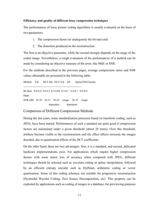
pixels with respect to a certain feature (e.g. grey level, texture); each region then has
some parameters related to the characterising feature associated with it.
The operations of finding a suitable segmentation and an optimum set of approximating
parameters are highly correlated, since the segmentation algorithm must take into account
the error produced by the region reconstruction (in order to limit this value within
determined bounds). These two operations constitute the logical modelling for this class
of coding schemes; quantisation and encoding are strongly dependent on the statistical
characteristics of the parameters of this approximation (and, therefore, on the
approximation itself).
Classical examples are polynomial approximation and texture approximation. For
polynomial approximation regions are reconstructed by means of polynomial functions in
(x, y); the task of the encoder is to find the optimum coefficients. In texture
approximation, regions are filled by synthesising a parametrised texture based on some
model (e.g. fractals, statistical methods, Markov Random Fields [MRF]). It must be
pointed out that, while in polynomial approximations the problem of finding optimum
coefficients is quite simple (it is possible to use least squares approximation or similar
exact formulations), for texture based techniques this problem can be very complex.
Spline approximation methods
These methodologies fall in the more general category of image reconstruction or sparse
8

9. data interpolation. The basic concept is to interpolate data from a set of points coming
from original pixel data or calculated in order to match some error criteria. The problem
of interpolating a set of sparse data is generally ill posed, so some regularization
algorithm must be adopted in order to obtain a unique solution. The problem is well
documented, and many interpolation algorithms have been proposed.
In order to apply this kind of technique to image coding, a good interpolant must be used
to match visual criteria. Spline interpolation provides a good visual interpolant,
notwithstanding its requiring a great computational effort. Bilinear interpolation is more
easy to implement, while maintaining a very good visual quality. Regularization involves
the minimisation of an energy function in order to obtain an interpolant which presents
some smoothness constraints; it can be combined with non-continuities along edges in
order to preserve contour quality during reconstruction. Generally all interpolants
computations require the solution of very large linear equation sets, even if related to
very sparse matrices. This leads to the use of recursive solution such as relaxation
(suitable for a large parallel implementation), or to the use of gradient descent algorithm.
Fractal coding :
Fractal parameters, including fractal dimension, lacunarity, as well as others described
below, have the potential to provide efficient methods of describing imagery in a highly
compact fashion for both intra- and interframe applications. Fractal methods have been
developed for both noisy and noise free coding methods.
Images of natural scenes are likely candidates because of the fractal structure of the scene
content, but results are reported to be applicable to a variety of binary, monochrome, and
colour scenes. Image compression algorithms which are noise free have been reported to
be developed from this transform for real time automatic image compression at ratios
between 10:1 and 100:1
Bit Allocation :
The first step in compressing an image is to segregate the image data into different
classes. Depending on the importance of the data it contains, each class is allocated a
portion of the total bit budget, such that the compressed image has the minimum possible
distortion. This procedure is called Bit Allocation.
9

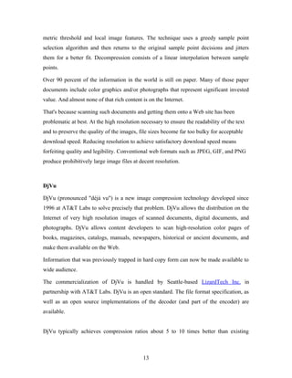
10. The Rate-Distortion theory is often used for solving the problem of allocating bits to a set
of classes, or for bit rate control in general. The theory aims at reducing the distortion for
a given target bit rate, by optimally allocating bits to the various classes of data. One
approach to solve the problem of Optimal Bit Allocation using the Rate-Distortion theory
is explained below.
Initially, all classes are allocated a predefined maximum number of bits.
For each class, one bit is reduced from its quota of allocated bits, and the distortion
due to the reduction of that 1 bit is calculated.
Of all the classes, the class with mininum distortion for a reduction of 1 bit is noted,
and 1 bit is reduced from its quota of bits.
The total distortion for all classes D is calculated.
The total rate for all the classes is calculated as: R = p(i) * B(i), where p is the
probability and B is the bit allocation for each class.
Compare the target rate and distortion specifications with the values obtained above.
If not optimal, go to step 2.
In the approach explained above, we keep on reducing one bit at a time till we achieve
optimality either in distortion or target rate, or both. An alternate approach which is also
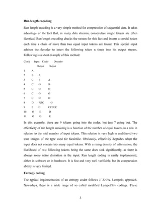
mentioned in [1] is to initially start with zero bits allocated for all classes, and to find the
class which is most 'benefitted' by getting an additional bit. The 'benefit' of a class is
defined as the decrease in distortion for that class.
Fig: 'Benefit' of a bit is the decrease in distortion due to receiving that bit.
As shown above, the benefit of a bit is a decreasing function of the number of bits
allocated previously to the same class. Both approaches mentioned above can be used to
the Bit Allocation problem.
10

11. Efficiency and quality of different lossy compression techniques
The performances of lossy picture coding algorithms is usually evaluated on the basis of
two parameters:
1. The compression factor (or analogously the bit rate) and
2. The distortion produced on the reconstruction.
The first is an objective parameter, while the second strongly depends on the usage of the
coded image. Nevertheless, a rough evaluation of the performances of a method can be
made by considering an objective measure of the error, like MSE or SNR.
For the methods described in the previous pages, average compression ratios and SNR
values obtainable are presented in the following table:
Method VQ DCT-SQ DCT-VQ AP SplineTSD Fractals
-------------------------------------------------------------------
Bit Rate 0.8-0.4 0.8-0.3 0.3-0.08 0.3-0.1 0.4-0.1 0.8-0.0
(bpp)
SNR (dB) 36-30 36-31 30-25 image 36-32 image
dependent dependent
Comparison of Different Compression Methods
During the last years, some standardisation processes based on transform coding, such as
JPEG, have been started. Performances of such a standard are quite good if compression
factors are maintained under a given threshold (about 20 times). Over this threshold,
artifacts become visible in the reconstruction and tile effect affects seriously the images
decoded, due to quantisation effects of the DCT coefficients.
On the other hand, there are two advantages: first, it is a standard, and second, dedicated
hardware implementations exist. For applications which require higher compression
factors with some minor loss of accuracy when compared with JPEG, different
techniques should be selected such as wavelets coding or spline interpolation, followed
by an efficient entropy encoder such as Huffman, arithmetic coding or vector
quantisation. Some of this coding schemes, are suitable for progressive reconstruction
(Pyramidal Wavelet Coding, Two Source Decomposition, etc). This property can be
exploited by applications such as coding of images in a database, for previewing purposes
11

12. or for transmission on a limited bandwidth channel.
Classifying image data
An image is represented as a two-dimentional array of coefficients, each coefficient
representing the brightness level in that point. When looking from a higher perspective,
we can't differentiate between coefficients as more important ones, and lesser important
ones. But thinking more intuitively, we can. Most natural images have smooth colour
variations, with the fine details being represented as sharp edges in between the smooth
variations. Technically, the smooth variations in colour can be termed as low frequency
variations and the sharp variations as high frequency variations.
The low frequency components (smooth variations) constitute the base of an image, and
the high frequency components (the edges which give the detail) add upon them to refine
the image, thereby giving a detailed image. Hence, the smooth variations are demanding
more importance than the details.
Separating the smooth variations and details of the image can be done in many ways. One
such way is the decomposition of the image using a Discrete Wavelet Transform (DWT).
Pyramidal Decomposition of Image
Non-Uniform Sampling and Interpolation for Lossy Image Compression
A set of experiments was performed with a lossy image compression algorithm that
utilizes non-uniform sampling and interpolation (NSI) of the image intensity surface. The
goal of this work was to create a lossy compression algorithm which was asymmetrical,
having a low decompression complexity and a potentially higher compression
complexity. The algorithm non-uniformly samples the image data in two dimensions. The
number of samples chosen, and hence the compression ratio, is based on a supplied error
12

13. metric threshold and local image features. The technique uses a greedy sample point
selection algorithm and then returns to the original sample point decisions and jitters
them for a better fit. Decompression consists of a linear interpolation between sample
points.
Over 90 percent of the information in the world is still on paper. Many of those paper
documents include color graphics and/or photographs that represent significant invested
value. And almost none of that rich content is on the Internet.
That's because scanning such documents and getting them onto a Web site has been
problematic at best. At the high resolution necessary to ensure the readability of the text
and to preserve the quality of the images, file sizes become far too bulky for acceptable
download speed. Reducing resolution to achieve satisfactory download speed means
forfeiting quality and legibility. Conventional web formats such as JPEG, GIF, and PNG
produce prohibitively large image files at decent resolution.
DjVu
DjVu (pronounced "déjà vu") is a new image compression technology developed since
1996 at AT&T Labs to solve precisely that problem. DjVu allows the distribution on the
Internet of very high resolution images of scanned documents, digital documents, and
photographs. DjVu allows content developers to scan high-resolution color pages of
books, magazines, catalogs, manuals, newspapers, historical or ancient documents, and
make them available on the Web.
Information that was previously trapped in hard copy form can now be made available to
wide audience.
The commercialization of DjVu is handled by Seattle-based LizardTech Inc. in
partnership with AT&T Labs. DjVu is an open standard. The file format specification, as
well as an open source implementations of the decoder (and part of the encoder) are
available.
DjVu typically achieves compression ratios about 5 to 10 times better than existing
13

14. methods such as JPEG and GIF for color documents, and 3 to 8 times than TIFF for black
and white documents. Scanned pages at 300 DPI in full color can be compressed down to
30 to 100KB files from 25MB.. Black-and-white pages at 300 DPI typically occupy 5 to
30KB when compressed. This puts the size of high-quality scanned pages within the
realm of an average HTML page (which is typically around 50KB).
For color document images that contain both text and pictures, DjVu files are typically 5
to 10 times smaller than JPEG at similar quality. For black-and-white pages, DjVu files
are typically 10 to 20 times smaller than JPEG and five times smaller than GIF. DjVu
files are also about 3 to 8 times smaller than black and white PDF files produced from
scanned documents (scanned documents in color are impractical in PDF).
In addition to scanned documents, DjVu can also be applied to documents produced
electronically in formats such as Adobe's PostScript or PDF. In that case, the file sizes are
between 15 to 20KB per page at 300 DPI..
The DjVu plug-in is available for standard Web browsers on various platforms. The
DjVu plug-in allows for easy panning and zooming of document images. A unique on the
fly decompression technology allows images that normally require 25MB of RAM to be
decompressed to require only 2MB of RAM.
Conventional image viewing software decompresses images in their entirety before
displaying them. This is impractical for high-resolution document images since they
typically go beyond the memory capacity of many PCs, causing excessive disk swapping.
DjVu, on the other hand, never decompresses the entire image, but instead keeps the
image in memory in a compact form, and decompresses the piece displayed on the screen
in real time as the user views the image. Images as large as 2,500 pixels by 3,300 pixels
(a standard page image at 300 DPI) can be downloaded and displayed on very low-end
PCs.
The DjVu format is progressive. Users get an initial version of the page very quickly, and
the visual quality of the page progressively improves as more bits arrive. For example,
the text of a typical magazine page would appear in just three seconds over a 56Kbps
modem connection. In another second or two, the first versions of the pictures and
backgrounds will appear. Then, after a few more seconds, the final full-quality version of
14

15. the page is completed.
One of the main technologies behind DjVu is the ability to separate an image into a
background layer (i.e., paper texture and pictures) and foreground layer (text and line
drawings). Traditional image compression techniques are fine for simple photographs,
but they drastically degrade sharp color transitions between adjacent highly contrasted
areas - which is why they render type so poorly. By separating the text from the
backgrounds, DjVu can keep the text at high resolution (thereby preserving the sharp
edges and maximizing legibility), while at the same time compressing the backgrounds
and pictures at lower resolution with a wavelet-based compression technique.
15

16. CONCLUSION
Image compression is the application of data compression or transmit data in an efficient
form. Image compression is minimizing the size in bytes of a graphics file without
degrading the quality of the image to an unaccceptable level. It also reduces the time
required for images to be sent over the Internet or downloaded from Web pages.There are
two categories of data compression algorithms: Lossless and Lossy
Reconstructing the image from the compressed data is usually a faster process than
compression.
16