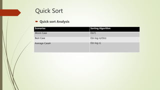
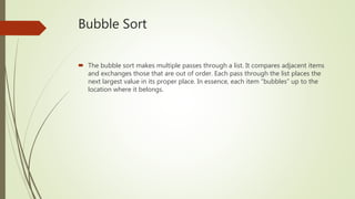
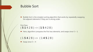
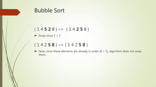
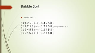
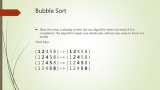
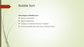
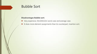
Quicksort is a recursive divide-and-conquer algorithm that works by selecting a pivot element and partitioning the array into two subarrays of elements less than and greater than the pivot. It recursively sorts the subarrays. The divide step does all the work by partitioning, while the combine step does nothing. It has average case performance of O(n log n) but worst case of O(n^2). Bubble sort repeatedly swaps adjacent elements that are out of order until the array is fully sorted. It has a simple implementation but poor performance of O(n^2).

![Quick Sort
Here is how quicksort uses divide-and-conquer: think of sorting a sub
array[p…r], Where initially the sub array is array[0…n-1].
We take this set of array as an example:
40 20 10 80 60 50 7 30 100
0 1 2 3 4 5 6 7 8](https://image.slidesharecdn.com/presentation-171213023732/85/Analysis-of-Algorithm-Bubblesort-and-Quicksort-3-320.jpg)
![Quick Sort
Divide
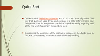
1. Choose any element in the sub array [p…r] call this element Pivot.
We now have our Pivot which is 40 at array 0
40 20 10 80 60 50 7 30 100
0 1 2 3 4 5 6 7 8](https://image.slidesharecdn.com/presentation-171213023732/85/Analysis-of-Algorithm-Bubblesort-and-Quicksort-4-320.jpg)
![Quick Sort
Given again the array
40 20 10 80 60 50 7 30 100
0 1 2 3 4 5 6 7 8
7 20 10 30 40 50 80 60 100
<= Data [pivot] > Data [pivot]](https://image.slidesharecdn.com/presentation-171213023732/85/Analysis-of-Algorithm-Bubblesort-and-Quicksort-6-320.jpg)
![Quick Sort
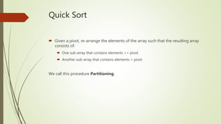
Conquer
After dividing recursively sort each sub array
<= Data [pivot]
7 20 10 30
7 20 10 30
7 20 10 30
7 10 20 30
7 20 10 30
7 10 20 30
7 10 20 30](https://image.slidesharecdn.com/presentation-171213023732/85/Analysis-of-Algorithm-Bubblesort-and-Quicksort-7-320.jpg)
![Quick Sort
Conquer
After dividing recursively sort each sub array
> Data [pivot]
50 60 80 100
50 80 60 100
50 80 60 100
50 80 60 100
50 60 80 100
50 80 60 100
50 60 80 100
50 60 80 100](https://image.slidesharecdn.com/presentation-171213023732/85/Analysis-of-Algorithm-Bubblesort-and-Quicksort-8-320.jpg)


![UNIT V Searching Sorting Hashing Techniques [Autosaved].pptx](https://cdn.slidesharecdn.com/ss_thumbnails/unitvsearchingsortinghashingtechniquesautosaved-241126054304-95a69c51-thumbnail.jpg?width=640&height=640&fit=bounds)
![UNIT V Searching Sorting Hashing Techniques [Autosaved].pptx](https://cdn.slidesharecdn.com/ss_thumbnails/unitvsearchingsortinghashingtechniquesautosaved-241014040608-74caa0f6-thumbnail.jpg?width=640&height=640&fit=bounds)