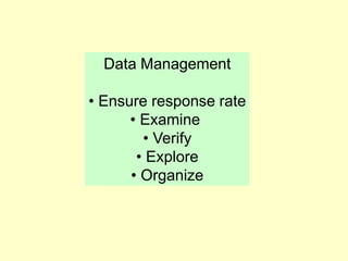
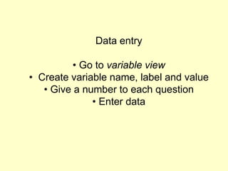
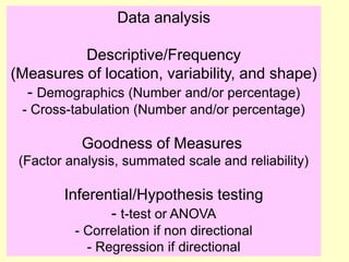
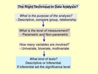
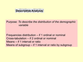
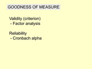
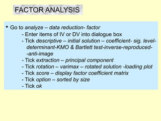
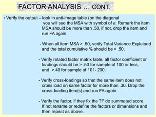
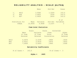
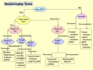
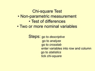
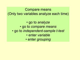
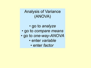
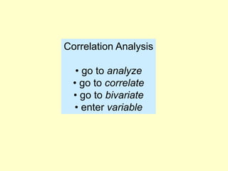
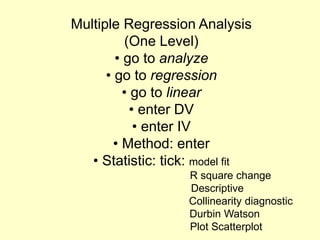
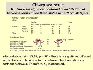
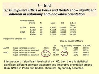
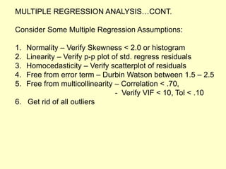
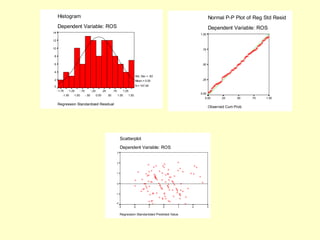
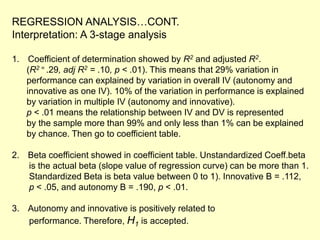
SlideShare a Scribd company logo
DATA ANALYSIS
For Management and
Marketing Research Project Report
SPSS 13.0
By:
Assoc Prof Dr Amran Awang
Faculty of Business Management
UiTM Perlis
Jan-May 2007
Objective:
• To know SPSS
• To manage data
• To enter and analyze data
• To interpret the findings
• To report the result
SPSS version 13.0
Statistical Package for Social Science
• User friendly
• Window orientation
• Use original copy
• Familiarity
Data Management
• Ensure response rate
• Examine
• Verify
• Explore
• Organize
Data entry
• Go to variable view
• Create variable name, label and value
• Give a number to each question
• Enter data
Data analysis
Descriptive/Frequency
(Measures of location, variability, and shape)
- Demographics (Number and/or percentage)
- Cross-tabulation (Number and/or percentage)
Goodness of Measures
(Factor analysis, summated scale and reliability)
Inferential/Hypothesis testing
- t-test or ANOVA
- Correlation if non directional
- Regression if directional
The Right Technique in Data Analysis?
What is the purpose of the analysis?
- Descriptive, compare group, relationship
What is the level of measurement?
- Parametric and Non-parametric
How many variables are involved?
- Univariate, bivariate, multivariate
What kind of tests?
Descriptive or Inferential.
If inferential set the significance level
Descriptive Analysis
Purpose: To describe the distribution of the demographic
variable
Frequencies distribution – if 1 ordinal or nominal
Cross-tabulation – if 2 ordinal or nominal
Means – if 1 interval or ratio
Means of subgroup – if 1 interval or ratio by subgroup
GOODNESS OF MEASURE
Validity (criterion)
- Factor analysis
Reliability
- Cronbach alpha
FACTOR ANALYSIS
• Go to analyze – data reduction- factor
- Enter items of IV or DV into dialogue box
- Tick descriptive – initial solution – coefficient- sig. level-
determinant-KMO & Bartlett test-inverse-reproduced-
-anti-image
- Tick extraction – principal component
- Tick rotation – varimax – rotated solution -loading plot
- Tick score – display factor coefficient matrix
- Tick option – sorted by size
- Tick ok
• Verify the output – look in anti-image table (on the diagonal
you will see the MSA with symbol of a. Remark the item
MSA should be more than .50, if not, drop the item and
run FA again.
- When all item MSA > .50, verify Total Variance Explained
and the total cumulative % should be > .50.
- Verify rotated factor matrix table, all factor coefficient or
loadings should be > .50 for sample of 100 or less,
and >.40 for sample of 101- 200.
- Verify cross-loadings so that the same item does not
cross load on same factor for more than .30. Drop the
cross-loading item(s) and run FA again.
- Verify the factor, if they fix the TF do summated score.
If not rename or redefine the factors or dimensions and
then repeat as above.
FACTOR ANALYSIS … CONT.
RELIABILITY
• Go to analyze – scale – reliability analysis
- Enter items to be analyzed
- Tick statistics – descriptive for –
item – scale – scale if item deleted.
• Verify the output
- If the scale (Cronbach alpha) > .70, the reliability
of the variable is achieved (Nunnally, 1978)
- If not verify the table and check the alpha
scale if item deleted to detect for improvement.
- Drop item stated in scale if item deleted and run
reliability again.
- Do summated scale to formulate a variable.
FACTOR ANALYSIS VS. RELIABILITY
If factor analysis does not in harmony with
reliability then go back to LR to confirm
the relationship found in previous studies
and how it was done.
KMO and Bartlett's Test
Kaiser-Meyer-Olkin Measure of Sampling Adequacy. .619
Bartlett's Test of Sphericity Approx. Chi-Square 327.667
df 91
Sig. .000
Total Variance Explained
Initial Eigenvalues Extraction Sums of Squared Loadings Rotation Sums of Squared Loadings
Component Total % of Variance Cumulative % Total % of Variance Cumulative % Total % of Variance Cumulative %
1 2.672 19.087 19.087 2.672 19.087 19.087 1.941 13.864 13.864
2 2.116 15.111 34.198 2.116 15.111 34.198 1.911 13.648 27.512
3 1.314 9.385 43.583 1.314 9.385 43.583 1.521 10.866 38.378
4 1.129 8.065 51.648 1.129 8.065 51.648 1.489 10.635 49.012
5 1.024 7.316 58.964 1.024 7.316 58.964 1.393 9.952 58.964
6 .915 6.538 65.502
7 .908 6.485 71.987
8 .820 5.860 77.848
9 .729 5.209 83.056
10 .628 4.484 87.540
11 .541 3.865 91.405
12 .471 3.365 94.771
13 .403 2.876 97.647
14 .329 2.353 100.000
Extraction Method: Principal Component Analysis.
Output of Factor Analysis
Rotated Component Matrix
Component
1 2 3 4 5
BO12 .742 6.966E-02 8.411E-02 .291 1.308E-02
BO7 .724 -5.468E-02 -.214 -8.570E-02 .146
BO6 .722 -1.121E-02 .243 .136 .129
BO8 6.309E-02 .801 .149 -4.440E-02 -4.116E-02
BO14 -.303 .772 .183 2.543E-02 .170
BO13 -.197 -.627 .137 .127 .333
BO11 -6.129E-02 8.341E-02 -.802 6.165E-02 .153
BO4 3.467E-02 .318 .599 9.943E-02 -7.414E-02
BO9 -1.251E-02 -1.622E-02 -1.564E-02 .820 5.378E-02
BO1 -.236 .230 .359 -.556 .143
BO2 .303 2.235E-02 .190 .539 .223
BO3 .196 .114 -3.516E-02 -9.854E-02 .797
BO10 -.127 .169 .212 -.214 -.577
BO5 4.868E-02 .260 .349 -.136 -.379
Extraction Method: Principal Component Analysis. Rotation Method: Varimax with
Kaiser Normalization. a Rotation converged in 6 iterations.
Output of Factor Analysis … cont.
R E L I A B I L I T Y A N A L Y S I S - S C A L E (A L P H A)
Mean Std Dev Cases
1. BO12 3.9580 1.0269 143.0
2. BO6 3.4825 .9704 143.0
3. BO7 2.9650 .8914 143.0
N of
Statistics for Mean Variance Std Dev Variables
SCALE 10.4056 4.9048 2.2147 3
Item-total Statistics
Scale Scale Corrected
Mean Variance Item- Alpha
if Item if Item Total if Item
Deleted Deleted Correlation Deleted
BO12 6.4476 2.3194 .4894 .5030
BO6 6.9231 2.4518 .4974 .4916
BO7 7.4406 2.9243 .3890 .6348
Reliability Coefficients
N of Cases = 143.0 N of Items = 3
Alpha = .6465
Test of Differences
Purpose: To evaluate the differences between 2 or
more groups with respect to a variable of interest
Techniques depended on:
• Levels of measurement of the variable
- Types of data (parametric or non-parametric)
• Number of groups
- One or more than two groups
• Independence of the groups
- If more than two groups
- Independence or related groups
INFERENTIAL
Test of Differences
One or
more than
2 groups
Independent
or related
One More than two groups
Independent
or related
Independent Related
Nominal: Frequency
Χ2 test
K-S
Runs
Binomial
Ordinal: Mann-Whitney
Continuous:
t-test
z-test
One-way ANOVA
Nominal:
Χ2 test
McNemar
Ordinal:
Wilcoxon
Sign
Rank
Continuous:
Paired t-test
Nominal:
Χ2 test
Ordinal:
Mann-Whitney
Median
K-S
Kruskal-Wallis
ANOVA
Continuous:
1-way ANOVA
Independent Related
Nominal:
Χ2 test
Ordinal:
Sign
Wilcoxon
McNemar
Friedman
2-way ANOVA
Continuous:
Paired t-test
Factorial
2-way ANOVA
Relationship
Purpose: To establish relationship between variables
Technique depended on:
• Whether or not exist dependent variable(s)
• Number of dependent and independent variables
• Types of data (parametric or non-parametric)
• Levels of measurement of the variable
Relationship Tests
One
Scale of
DV
Parametric
Scale of
IV
Parametric
Multiple
Regression
Analysis
(MRA)
Non-parametric
MRA w/
dummy
Loglinear
Scale
of IV
Non-parametric
Conjoint
analysis
Non-parametric
Scale
of IV
Parametric
Discriminant
Analysis
Logit & probit
Scale of
DV
More than 1
Scale
of IV
Parametric
Parametric Non-parametric
Canonical
Correlation
LISREL
Multivariate
ANOVA
Any DV?
Yes
No
Variable
Cluster
analysis
Factor
Analysis
MDS
Factor
Analysis
Latent
Structure
MDS
Cluster
analysis
Parametric Non-parametric
How many
DV?
Chi-square Test
• Non-parametric measurement
• Test of differences
• Two or more nominal variables
Steps: go to descriptive
go to analyze
go to crosstab
enter variables into row and column
go to statistics
tick chi-square
Compare means
(Only two variables analyze each time)
• go to analyze
• go to compare means
• go to independent-sample t-test
• enter variable
• enter grouping
Analysis of Variance
(ANOVA)
• go to analyze
• go to compare means
• go to one-way-ANOVA
• enter variable
• enter factor
Correlation Analysis
• go to analyze
• go to correlate
• go to bivariate
• enter variable
Multiple Regression Analysis
(One Level)
• go to analyze
• go to regression
• go to linear
• enter DV
• enter IV
• Method: enter
• Statistic: tick: model fit
R square change
Descriptive
Collinearity diagnostic
Durbin Watson
Plot Scatterplot
Chi-square result
H1: There are significant different in distribution of
business forms in the three states in northern Malaysia
STATE * FORM Crosstabulation
Count
FORM Total
Proprietor Partnership Pte Ltd Ltd
STATE Perlis 12 5 28 1 46
Kedah 51 16 31 1 99
Penang 20 16 24 5 65
Total 83 37 83 7 210
Chi-Square Tests
Value df Asymp. Sig. (2-sided)
Pearson Chi-Square 22.675 6 .001
Likelihood Ratio 21.745 6 .001
Linear-by-Linear Association .275 1 .600
N of Valid Cases 210
a 3 cells (25.0%) have expected count less than 5. The minimum expected count is 1.53.
Interpretation: (2 = 22.67, p < .01), there is a significant different
in distribution of business forms between the three states in
northern Malaysia. Therefore, H1 is accepted.
Group Statistics
STATE N Mean SD S. E. of
Mean
AUTO Perlis 46 1.3696 .48802 .07195
Kedah 99 1.5051 .50252 .05051
INNO Perlis 46 1.5435 .50361 .07425
Kedah 99 1.7677 .42446 .04266
Independent Samples Test
t-test for Equality of Means
t df Sig. (2-tailed) Mean Diff. S. E. Diff.
AUTO Equal variances assumed -1.525 143 .130 -.1355 .08886
Equal variances not assumed -1.541 90.208 .127 -.1355 .08791
INNO Equal variances assumed -2.787 143 .006 -.2242 .08045
Equal variances not assumed -2.618 75.817 .011 -.2242 .08564
t – test
H1: Bumiputera SMEs in Perlis and Kedah show significant
different in autonomy and innovative orientation
Interpretation: If significant level set at p < .05, then there is statistical
significant different between autonomy and innovative orientation among
Bumi SMEs in Perlis and Kedah. Therefore, H1 partially accepted.
ANOVA
H1: There is significant different in autonomy and innovative
orientation among Bumiputera SMEs in the three
states in northern Malaysia
Sum of Squares df Mean Square F Sig.
AUTO Between Groups .749 2 .375 1.519 .221
Within Groups 51.065 207 .247
Total 51.814 209
INNO Between Groups 4.393 2 2.196 10.074 .000
Within Groups 45.131 207 .218
Total 49.524 209
Interpretation:
(F = 10.074, p < .01). If significant level is set at p < .05, then
there is statistical significant different in innovative but not
statistical significant in autonomy orientation among Bumi SMEs
in the three states in Northern Malaysia.
Therefore, H1 is partially accepted.
Correlation
H1: Autonomy and innovative orientation among Bumiputera
SMEs in northern Malaysia are related significantly
Correlations
Autonomy Innovative
Autonomy Pearson Correlation 1 .072
Sig. (2-tailed) . .297
N 210 210
Innovative Pearson Correlation .072 1
Sig. (2-tailed) .297 .
N 210 210
Interpretation:
(r = .072, p < .297) if significant level is set at p < .05, then
there is no statistical significant correlation between autonomy
and innovativeness. Therefore, H1 rejected.
Interpretation of Findings
Statistics
Autonomy Innovative
N Valid 210 210
Missing 0 0
Mean 3.0444 5.6603
Median 3.0000 6.0000
Mode 2.00 6.00
Std. Deviation 1.21533 .97658
Skewness .458 -.908
Std. Error of Skewness .168 .168
Kurtosis -.225 1.057
Std. Error of Kurtosis .334 .334
Minimum 1.00 2.00
Maximum 7.00 7.00
a Multiple modes exist. The smallest value is shown
STATE
Frequency % Valid % Cumulative %
Valid Perlis 46 21.9 21.9 21.9
Kedah 99 47.1 47.1 69.0
Penang 65 31.0 31.0 100.0
Total 210 100.0 100.0
Multiple Regression Analysis
H1: Autonomy and innovative orientation are positively related to
performance among Bumiputera SMEs in northern Malaysia
Model Summary
R R Square Adj R Square S. E. E. Change Statistics
Model R Sq Chg F Change df1 df2 Sig. F Chg
1 .171 .29 .10 1.52865 .026 2.730 2 205 .008
a Predictors: (Constant), Autonomy Dimension, Innovativeness Dimension
Coefficients
Ustd Coef. Std Coef. t Sig. Coll Stat
Model B S. E. Beta Tolerance VIF
1 (Constant) 4.053 .752 5.390 .000
Innovative .112 .113 .071 1.989 .024 .911 1.098
Autonomy .190 .090 .151 2.126 .005 .944 1.059
a Dependent Variable: Performance
MULTIPLE REGRESSION ANALYSIS…CONT.
Consider Some Multiple Regression Assumptions:
1. Normality – Verify Skewness < 2.0 or histogram
2. Linearity – Verify p-p plot of std. regress residuals
3. Homocedasticity – Verify scatterplot of residuals
4. Free from error term – Durbin Watson between 1.5 – 2.5
5. Free from multicollinearity – Correlation < .70,
- Verify VIF < 10, Tol < .10
6. Get rid of all outliers
Normal P-P Plot of Reg Std Resid
Dependent Variable: ROS
Observed Cum Prob
1.00
.75
.50
.25
0.00
Expected
Cum
Prob
1.00
.75
.50
.25
0.00
Scatterplot
Dependent Variable: ROS
Regression Standardized Predicted Value
3
2
1
0
-1
-2
-3
Regression
Studentized
Residual
3
2
1
0
-1
-2
Regression Standardized Residual
1.50
1.25
1.00
.75
.50
.25
0.00
-.25
-.50
-.75
-1.00
-1.25
-1.50
-1.75
Histogram
Dependent Variable: ROS
Frequency
14
12
10
8
6
4
2
0
Std. Dev = .83
Mean = 0.00
N = 107.00
REGRESSION ANALYSIS…CONT.
Interpretation: A 3-stage analysis
1. Coefficient of determination showed by R2 and adjusted R2.
(R2 = .29, adj R2 = .10, p < .01). This means that 29% variation in
performance can explained by variation in overall IV (autonomy and
innovative as one IV). 10% of the variation in performance is explained
by variation in multiple IV (autonomy and innovative).
p < .01 means the relationship between IV and DV is represented
by the sample more than 99% and only less than 1% can be explained
by chance. Then go to coefficient table.
2. Beta coefficient showed in coefficient table. Unstandardized Coeff.beta
is the actual beta (slope value of regression curve) can be more than 1.
Standardized Beta is beta value between 0 to 1). Innovative B = .112,
p < .05, and autonomy B = .190, p < .01.
3. Autonomy and innovative is positively related to
performance. Therefore, H1 is accepted.
THANK YOU ALL
Now analyze your own data

More Related Content

Similar to Data_Analysis_SPSS_Technique.ppt

Aminullah assagaf model regresi lengkap 10 agustus 2021_(sobel, path, outlier)
Aminullah assagaf model regresi lengkap  10 agustus 2021_(sobel, path, outlier)Aminullah assagaf model regresi lengkap  10 agustus 2021_(sobel, path, outlier)
Aminullah assagaf model regresi lengkap 10 agustus 2021_(sobel, path, outlier)
Aminullah Assagaf
 
Aminullah assagaf model regresi lengkap 17 okt 2021_(sobel, path, outlier)
Aminullah assagaf model regresi lengkap  17 okt 2021_(sobel, path, outlier)Aminullah assagaf model regresi lengkap  17 okt 2021_(sobel, path, outlier)
Aminullah assagaf model regresi lengkap 17 okt 2021_(sobel, path, outlier)
Aminullah Assagaf
 
Aminullah assagaf model regresi lengkap 10 agustus 2021_(sobel, path, outlier)
Aminullah assagaf model regresi lengkap  10 agustus 2021_(sobel, path, outlier)Aminullah assagaf model regresi lengkap  10 agustus 2021_(sobel, path, outlier)
Aminullah assagaf model regresi lengkap 10 agustus 2021_(sobel, path, outlier)
Aminullah Assagaf
 
Aminullah assagaf model regresi 17+ 5 des 2021
Aminullah assagaf model regresi 17+ 5 des 2021Aminullah assagaf model regresi 17+ 5 des 2021
Aminullah assagaf model regresi 17+ 5 des 2021
Aminullah Assagaf
 
Aminullah assagaf model regresi 17+ 5 des 2021
Aminullah assagaf model regresi 17+ 5 des 2021Aminullah assagaf model regresi 17+ 5 des 2021
Aminullah assagaf model regresi 17+ 5 des 2021
Aminullah Assagaf
 
Missing Parts I don’t think you understood the assignment.docx
Missing Parts I don’t think you understood the assignment.docxMissing Parts I don’t think you understood the assignment.docx
Missing Parts I don’t think you understood the assignment.docx
annandleola
 
Measure of dispersion by Neeraj Bhandari ( Surkhet.Nepal )
Measure of dispersion by Neeraj Bhandari ( Surkhet.Nepal )Measure of dispersion by Neeraj Bhandari ( Surkhet.Nepal )
Measure of dispersion by Neeraj Bhandari ( Surkhet.Nepal )
Neeraj Bhandari
 

Similar to Data_Analysis_SPSS_Technique.ppt (20)

Aminullah assagaf model regresi lengkap 10 agustus 2021_(sobel, path, outlier)
Aminullah assagaf model regresi lengkap  10 agustus 2021_(sobel, path, outlier)Aminullah assagaf model regresi lengkap  10 agustus 2021_(sobel, path, outlier)
Aminullah assagaf model regresi lengkap 10 agustus 2021_(sobel, path, outlier)
 
Aminullah assagaf model regresi lengkap 17 okt 2021_(sobel, path, outlier)
Aminullah assagaf model regresi lengkap  17 okt 2021_(sobel, path, outlier)Aminullah assagaf model regresi lengkap  17 okt 2021_(sobel, path, outlier)
Aminullah assagaf model regresi lengkap 17 okt 2021_(sobel, path, outlier)
 
Types of graphs
Types of graphsTypes of graphs
Types of graphs
 
Aminullah assagaf model regresi lengkap 10 agustus 2021_(sobel, path, outlier)
Aminullah assagaf model regresi lengkap  10 agustus 2021_(sobel, path, outlier)Aminullah assagaf model regresi lengkap  10 agustus 2021_(sobel, path, outlier)
Aminullah assagaf model regresi lengkap 10 agustus 2021_(sobel, path, outlier)
 
Measures of Dispersion.pptx
Measures of Dispersion.pptxMeasures of Dispersion.pptx
Measures of Dispersion.pptx
 
Aminullah assagaf model regresi 17+ 5 des 2021
Aminullah assagaf model regresi 17+ 5 des 2021Aminullah assagaf model regresi 17+ 5 des 2021
Aminullah assagaf model regresi 17+ 5 des 2021
 
Aminullah assagaf regresi17
Aminullah assagaf regresi17Aminullah assagaf regresi17
Aminullah assagaf regresi17
 
Aminullah assagaf model regresi 17+ 5 des 2021
Aminullah assagaf model regresi 17+ 5 des 2021Aminullah assagaf model regresi 17+ 5 des 2021
Aminullah assagaf model regresi 17+ 5 des 2021
 
Aminullah assagaf regresi17
Aminullah assagaf regresi17Aminullah assagaf regresi17
Aminullah assagaf regresi17
 
UNIT IV.pptx
UNIT IV.pptxUNIT IV.pptx
UNIT IV.pptx
 
Missing Parts I don’t think you understood the assignment.docx
Missing Parts I don’t think you understood the assignment.docxMissing Parts I don’t think you understood the assignment.docx
Missing Parts I don’t think you understood the assignment.docx
 
PILOT STUDY RESULTS TURNAROUND - EDITED.pptx
PILOT STUDY RESULTS TURNAROUND - EDITED.pptxPILOT STUDY RESULTS TURNAROUND - EDITED.pptx
PILOT STUDY RESULTS TURNAROUND - EDITED.pptx
 
Simple rules for building robust machine learning models
Simple rules for building robust machine learning modelsSimple rules for building robust machine learning models
Simple rules for building robust machine learning models
 
Intro to data science
Intro to data scienceIntro to data science
Intro to data science
 
Introduction To Data Science Using R
Introduction To Data Science Using RIntroduction To Data Science Using R
Introduction To Data Science Using R
 
Factor Analysis for Exploratory Studies
Factor Analysis for Exploratory StudiesFactor Analysis for Exploratory Studies
Factor Analysis for Exploratory Studies
 
Measure of central tendency
Measure of central tendency Measure of central tendency
Measure of central tendency
 
Exploratory factor analysis
Exploratory factor analysisExploratory factor analysis
Exploratory factor analysis
 
Measure of dispersion by Neeraj Bhandari ( Surkhet.Nepal )
Measure of dispersion by Neeraj Bhandari ( Surkhet.Nepal )Measure of dispersion by Neeraj Bhandari ( Surkhet.Nepal )
Measure of dispersion by Neeraj Bhandari ( Surkhet.Nepal )
 
Basic Statistics for Paid Search Advertising
Basic Statistics for Paid Search AdvertisingBasic Statistics for Paid Search Advertising
Basic Statistics for Paid Search Advertising
 

More from RiyadhJack

Roger LeRoy Miller, Daniel K. Benjamin - The Economics of Macro Issues-Pearso...
Roger LeRoy Miller, Daniel K. Benjamin - The Economics of Macro Issues-Pearso...Roger LeRoy Miller, Daniel K. Benjamin - The Economics of Macro Issues-Pearso...
Roger LeRoy Miller, Daniel K. Benjamin - The Economics of Macro Issues-Pearso...
RiyadhJack
 
L-14 Modeling Strategies and Policy Analysis - NR.pptx
L-14 Modeling Strategies and Policy Analysis - NR.pptxL-14 Modeling Strategies and Policy Analysis - NR.pptx
L-14 Modeling Strategies and Policy Analysis - NR.pptx
RiyadhJack
 
L11 - Forecasting and Smoothing using the Kalman Filter.pptx
L11 - Forecasting and Smoothing using the Kalman Filter.pptxL11 - Forecasting and Smoothing using the Kalman Filter.pptx
L11 - Forecasting and Smoothing using the Kalman Filter.pptx
RiyadhJack
 
L-8 VECM Formulation, Hypothesis Testing, and Forecasting - KH.pptx
L-8 VECM Formulation, Hypothesis Testing, and Forecasting - KH.pptxL-8 VECM Formulation, Hypothesis Testing, and Forecasting - KH.pptx
L-8 VECM Formulation, Hypothesis Testing, and Forecasting - KH.pptx
RiyadhJack
 
Mehwar_Consulting_quarterly_economic_bulletin_1631225461.pdf
Mehwar_Consulting_quarterly_economic_bulletin_1631225461.pdfMehwar_Consulting_quarterly_economic_bulletin_1631225461.pdf
Mehwar_Consulting_quarterly_economic_bulletin_1631225461.pdf
RiyadhJack
 

More from RiyadhJack (9)

Roger LeRoy Miller, Daniel K. Benjamin - The Economics of Macro Issues-Pearso...
Roger LeRoy Miller, Daniel K. Benjamin - The Economics of Macro Issues-Pearso...Roger LeRoy Miller, Daniel K. Benjamin - The Economics of Macro Issues-Pearso...
Roger LeRoy Miller, Daniel K. Benjamin - The Economics of Macro Issues-Pearso...
 
L-14 Modeling Strategies and Policy Analysis - NR.pptx
L-14 Modeling Strategies and Policy Analysis - NR.pptxL-14 Modeling Strategies and Policy Analysis - NR.pptx
L-14 Modeling Strategies and Policy Analysis - NR.pptx
 
L11 - Forecasting and Smoothing using the Kalman Filter.pptx
L11 - Forecasting and Smoothing using the Kalman Filter.pptxL11 - Forecasting and Smoothing using the Kalman Filter.pptx
L11 - Forecasting and Smoothing using the Kalman Filter.pptx
 
L-8 VECM Formulation, Hypothesis Testing, and Forecasting - KH.pptx
L-8 VECM Formulation, Hypothesis Testing, and Forecasting - KH.pptxL-8 VECM Formulation, Hypothesis Testing, and Forecasting - KH.pptx
L-8 VECM Formulation, Hypothesis Testing, and Forecasting - KH.pptx
 
Mehwar_Consulting_quarterly_economic_bulletin_1631225461.pdf
Mehwar_Consulting_quarterly_economic_bulletin_1631225461.pdfMehwar_Consulting_quarterly_economic_bulletin_1631225461.pdf
Mehwar_Consulting_quarterly_economic_bulletin_1631225461.pdf
 
1. CGE_overview.pptx
1. CGE_overview.pptx1. CGE_overview.pptx
1. CGE_overview.pptx
 
2. Recap - GAMS.pptx
2. Recap - GAMS.pptx2. Recap - GAMS.pptx
2. Recap - GAMS.pptx
 
Value_Chain_Analysis.pptx
Value_Chain_Analysis.pptxValue_Chain_Analysis.pptx
Value_Chain_Analysis.pptx
 
EViews_Student_Version_ppt.ppt
EViews_Student_Version_ppt.pptEViews_Student_Version_ppt.ppt
EViews_Student_Version_ppt.ppt
 

Recently uploaded

Computer Presentation.pptx ecommerce advantage s
Computer Presentation.pptx ecommerce advantage sComputer Presentation.pptx ecommerce advantage s
Computer Presentation.pptx ecommerce advantage s
MAQIB18
 
Professional Data Engineer Certification Exam Guide  _  Learn  _  Google Clou...
Professional Data Engineer Certification Exam Guide  _  Learn  _  Google Clou...Professional Data Engineer Certification Exam Guide  _  Learn  _  Google Clou...
Professional Data Engineer Certification Exam Guide  _  Learn  _  Google Clou...
Domenico Conte
 
一比一原版(UPenn毕业证)宾夕法尼亚大学毕业证成绩单
一比一原版(UPenn毕业证)宾夕法尼亚大学毕业证成绩单一比一原版(UPenn毕业证)宾夕法尼亚大学毕业证成绩单
一比一原版(UPenn毕业证)宾夕法尼亚大学毕业证成绩单
ewymefz
 
一比一原版(BU毕业证)波士顿大学毕业证成绩单
一比一原版(BU毕业证)波士顿大学毕业证成绩单一比一原版(BU毕业证)波士顿大学毕业证成绩单
一比一原版(BU毕业证)波士顿大学毕业证成绩单
ewymefz
 
一比一原版(CBU毕业证)卡普顿大学毕业证成绩单
一比一原版(CBU毕业证)卡普顿大学毕业证成绩单一比一原版(CBU毕业证)卡普顿大学毕业证成绩单
一比一原版(CBU毕业证)卡普顿大学毕业证成绩单
nscud
 
一比一原版(UMich毕业证)密歇根大学|安娜堡分校毕业证成绩单
一比一原版(UMich毕业证)密歇根大学|安娜堡分校毕业证成绩单一比一原版(UMich毕业证)密歇根大学|安娜堡分校毕业证成绩单
一比一原版(UMich毕业证)密歇根大学|安娜堡分校毕业证成绩单
ewymefz
 
一比一原版(TWU毕业证)西三一大学毕业证成绩单
一比一原版(TWU毕业证)西三一大学毕业证成绩单一比一原版(TWU毕业证)西三一大学毕业证成绩单
一比一原版(TWU毕业证)西三一大学毕业证成绩单
ocavb
 
standardisation of garbhpala offhgfffghh
standardisation of garbhpala offhgfffghhstandardisation of garbhpala offhgfffghh
standardisation of garbhpala offhgfffghh
ArpitMalhotra16
 
Opendatabay - Open Data Marketplace.pptx
Opendatabay - Open Data Marketplace.pptxOpendatabay - Open Data Marketplace.pptx
Opendatabay - Open Data Marketplace.pptx
Opendatabay
 
一比一原版(YU毕业证)约克大学毕业证成绩单
一比一原版(YU毕业证)约克大学毕业证成绩单一比一原版(YU毕业证)约克大学毕业证成绩单
一比一原版(YU毕业证)约克大学毕业证成绩单
enxupq
 
一比一原版(RUG毕业证)格罗宁根大学毕业证成绩单
一比一原版(RUG毕业证)格罗宁根大学毕业证成绩单一比一原版(RUG毕业证)格罗宁根大学毕业证成绩单
一比一原版(RUG毕业证)格罗宁根大学毕业证成绩单
vcaxypu
 

Recently uploaded (20)

Computer Presentation.pptx ecommerce advantage s
Computer Presentation.pptx ecommerce advantage sComputer Presentation.pptx ecommerce advantage s
Computer Presentation.pptx ecommerce advantage s
 
Professional Data Engineer Certification Exam Guide  _  Learn  _  Google Clou...
Professional Data Engineer Certification Exam Guide  _  Learn  _  Google Clou...Professional Data Engineer Certification Exam Guide  _  Learn  _  Google Clou...
Professional Data Engineer Certification Exam Guide  _  Learn  _  Google Clou...
 
Q1’2024 Update: MYCI’s Leap Year Rebound
Q1’2024 Update: MYCI’s Leap Year ReboundQ1’2024 Update: MYCI’s Leap Year Rebound
Q1’2024 Update: MYCI’s Leap Year Rebound
 
一比一原版(UPenn毕业证)宾夕法尼亚大学毕业证成绩单
一比一原版(UPenn毕业证)宾夕法尼亚大学毕业证成绩单一比一原版(UPenn毕业证)宾夕法尼亚大学毕业证成绩单
一比一原版(UPenn毕业证)宾夕法尼亚大学毕业证成绩单
 
Criminal IP - Threat Hunting Webinar.pdf
Criminal IP - Threat Hunting Webinar.pdfCriminal IP - Threat Hunting Webinar.pdf
Criminal IP - Threat Hunting Webinar.pdf
 
一比一原版(BU毕业证)波士顿大学毕业证成绩单
一比一原版(BU毕业证)波士顿大学毕业证成绩单一比一原版(BU毕业证)波士顿大学毕业证成绩单
一比一原版(BU毕业证)波士顿大学毕业证成绩单
 
tapal brand analysis PPT slide for comptetive data
tapal brand analysis PPT slide for comptetive datatapal brand analysis PPT slide for comptetive data
tapal brand analysis PPT slide for comptetive data
 
Criminal IP - Threat Hunting Webinar.pdf
Criminal IP - Threat Hunting Webinar.pdfCriminal IP - Threat Hunting Webinar.pdf
Criminal IP - Threat Hunting Webinar.pdf
 
Innovative Methods in Media and Communication Research by Sebastian Kubitschk...
Innovative Methods in Media and Communication Research by Sebastian Kubitschk...Innovative Methods in Media and Communication Research by Sebastian Kubitschk...
Innovative Methods in Media and Communication Research by Sebastian Kubitschk...
 
一比一原版(CBU毕业证)卡普顿大学毕业证成绩单
一比一原版(CBU毕业证)卡普顿大学毕业证成绩单一比一原版(CBU毕业证)卡普顿大学毕业证成绩单
一比一原版(CBU毕业证)卡普顿大学毕业证成绩单
 
Using PDB Relocation to Move a Single PDB to Another Existing CDB
Using PDB Relocation to Move a Single PDB to Another Existing CDBUsing PDB Relocation to Move a Single PDB to Another Existing CDB
Using PDB Relocation to Move a Single PDB to Another Existing CDB
 
一比一原版(UMich毕业证)密歇根大学|安娜堡分校毕业证成绩单
一比一原版(UMich毕业证)密歇根大学|安娜堡分校毕业证成绩单一比一原版(UMich毕业证)密歇根大学|安娜堡分校毕业证成绩单
一比一原版(UMich毕业证)密歇根大学|安娜堡分校毕业证成绩单
 
一比一原版(TWU毕业证)西三一大学毕业证成绩单
一比一原版(TWU毕业证)西三一大学毕业证成绩单一比一原版(TWU毕业证)西三一大学毕业证成绩单
一比一原版(TWU毕业证)西三一大学毕业证成绩单
 
standardisation of garbhpala offhgfffghh
standardisation of garbhpala offhgfffghhstandardisation of garbhpala offhgfffghh
standardisation of garbhpala offhgfffghh
 
Opendatabay - Open Data Marketplace.pptx
Opendatabay - Open Data Marketplace.pptxOpendatabay - Open Data Marketplace.pptx
Opendatabay - Open Data Marketplace.pptx
 
社内勉強会資料_LLM Agents                              .
社内勉強会資料_LLM Agents                              .社内勉強会資料_LLM Agents                              .
社内勉強会資料_LLM Agents                              .
 
Business update Q1 2024 Lar España Real Estate SOCIMI
Business update Q1 2024 Lar España Real Estate SOCIMIBusiness update Q1 2024 Lar España Real Estate SOCIMI
Business update Q1 2024 Lar España Real Estate SOCIMI
 
一比一原版(YU毕业证)约克大学毕业证成绩单
一比一原版(YU毕业证)约克大学毕业证成绩单一比一原版(YU毕业证)约克大学毕业证成绩单
一比一原版(YU毕业证)约克大学毕业证成绩单
 
Jpolillo Amazon PPC - Bid Optimization Sample
Jpolillo Amazon PPC - Bid Optimization SampleJpolillo Amazon PPC - Bid Optimization Sample
Jpolillo Amazon PPC - Bid Optimization Sample
 
一比一原版(RUG毕业证)格罗宁根大学毕业证成绩单
一比一原版(RUG毕业证)格罗宁根大学毕业证成绩单一比一原版(RUG毕业证)格罗宁根大学毕业证成绩单
一比一原版(RUG毕业证)格罗宁根大学毕业证成绩单
 

Data_Analysis_SPSS_Technique.ppt

  • 1. DATA ANALYSIS For Management and Marketing Research Project Report SPSS 13.0 By: Assoc Prof Dr Amran Awang Faculty of Business Management UiTM Perlis Jan-May 2007
  • 2. Objective: • To know SPSS • To manage data • To enter and analyze data • To interpret the findings • To report the result
  • 3. SPSS version 13.0 Statistical Package for Social Science • User friendly • Window orientation • Use original copy • Familiarity
  • 4. Data Management • Ensure response rate • Examine • Verify • Explore • Organize
  • 5. Data entry • Go to variable view • Create variable name, label and value • Give a number to each question • Enter data
  • 6. Data analysis Descriptive/Frequency (Measures of location, variability, and shape) - Demographics (Number and/or percentage) - Cross-tabulation (Number and/or percentage) Goodness of Measures (Factor analysis, summated scale and reliability) Inferential/Hypothesis testing - t-test or ANOVA - Correlation if non directional - Regression if directional
  • 7. The Right Technique in Data Analysis? What is the purpose of the analysis? - Descriptive, compare group, relationship What is the level of measurement? - Parametric and Non-parametric How many variables are involved? - Univariate, bivariate, multivariate What kind of tests? Descriptive or Inferential. If inferential set the significance level
  • 8. Descriptive Analysis Purpose: To describe the distribution of the demographic variable Frequencies distribution – if 1 ordinal or nominal Cross-tabulation – if 2 ordinal or nominal Means – if 1 interval or ratio Means of subgroup – if 1 interval or ratio by subgroup
  • 9. GOODNESS OF MEASURE Validity (criterion) - Factor analysis Reliability - Cronbach alpha
  • 10. FACTOR ANALYSIS • Go to analyze – data reduction- factor - Enter items of IV or DV into dialogue box - Tick descriptive – initial solution – coefficient- sig. level- determinant-KMO & Bartlett test-inverse-reproduced- -anti-image - Tick extraction – principal component - Tick rotation – varimax – rotated solution -loading plot - Tick score – display factor coefficient matrix - Tick option – sorted by size - Tick ok
  • 11. • Verify the output – look in anti-image table (on the diagonal you will see the MSA with symbol of a. Remark the item MSA should be more than .50, if not, drop the item and run FA again. - When all item MSA > .50, verify Total Variance Explained and the total cumulative % should be > .50. - Verify rotated factor matrix table, all factor coefficient or loadings should be > .50 for sample of 100 or less, and >.40 for sample of 101- 200. - Verify cross-loadings so that the same item does not cross load on same factor for more than .30. Drop the cross-loading item(s) and run FA again. - Verify the factor, if they fix the TF do summated score. If not rename or redefine the factors or dimensions and then repeat as above. FACTOR ANALYSIS … CONT.
  • 12. RELIABILITY • Go to analyze – scale – reliability analysis - Enter items to be analyzed - Tick statistics – descriptive for – item – scale – scale if item deleted. • Verify the output - If the scale (Cronbach alpha) > .70, the reliability of the variable is achieved (Nunnally, 1978) - If not verify the table and check the alpha scale if item deleted to detect for improvement. - Drop item stated in scale if item deleted and run reliability again. - Do summated scale to formulate a variable.
  • 13. FACTOR ANALYSIS VS. RELIABILITY If factor analysis does not in harmony with reliability then go back to LR to confirm the relationship found in previous studies and how it was done.
  • 14. KMO and Bartlett's Test Kaiser-Meyer-Olkin Measure of Sampling Adequacy. .619 Bartlett's Test of Sphericity Approx. Chi-Square 327.667 df 91 Sig. .000 Total Variance Explained Initial Eigenvalues Extraction Sums of Squared Loadings Rotation Sums of Squared Loadings Component Total % of Variance Cumulative % Total % of Variance Cumulative % Total % of Variance Cumulative % 1 2.672 19.087 19.087 2.672 19.087 19.087 1.941 13.864 13.864 2 2.116 15.111 34.198 2.116 15.111 34.198 1.911 13.648 27.512 3 1.314 9.385 43.583 1.314 9.385 43.583 1.521 10.866 38.378 4 1.129 8.065 51.648 1.129 8.065 51.648 1.489 10.635 49.012 5 1.024 7.316 58.964 1.024 7.316 58.964 1.393 9.952 58.964 6 .915 6.538 65.502 7 .908 6.485 71.987 8 .820 5.860 77.848 9 .729 5.209 83.056 10 .628 4.484 87.540 11 .541 3.865 91.405 12 .471 3.365 94.771 13 .403 2.876 97.647 14 .329 2.353 100.000 Extraction Method: Principal Component Analysis. Output of Factor Analysis
  • 15. Rotated Component Matrix Component 1 2 3 4 5 BO12 .742 6.966E-02 8.411E-02 .291 1.308E-02 BO7 .724 -5.468E-02 -.214 -8.570E-02 .146 BO6 .722 -1.121E-02 .243 .136 .129 BO8 6.309E-02 .801 .149 -4.440E-02 -4.116E-02 BO14 -.303 .772 .183 2.543E-02 .170 BO13 -.197 -.627 .137 .127 .333 BO11 -6.129E-02 8.341E-02 -.802 6.165E-02 .153 BO4 3.467E-02 .318 .599 9.943E-02 -7.414E-02 BO9 -1.251E-02 -1.622E-02 -1.564E-02 .820 5.378E-02 BO1 -.236 .230 .359 -.556 .143 BO2 .303 2.235E-02 .190 .539 .223 BO3 .196 .114 -3.516E-02 -9.854E-02 .797 BO10 -.127 .169 .212 -.214 -.577 BO5 4.868E-02 .260 .349 -.136 -.379 Extraction Method: Principal Component Analysis. Rotation Method: Varimax with Kaiser Normalization. a Rotation converged in 6 iterations. Output of Factor Analysis … cont.
  • 16. R E L I A B I L I T Y A N A L Y S I S - S C A L E (A L P H A) Mean Std Dev Cases 1. BO12 3.9580 1.0269 143.0 2. BO6 3.4825 .9704 143.0 3. BO7 2.9650 .8914 143.0 N of Statistics for Mean Variance Std Dev Variables SCALE 10.4056 4.9048 2.2147 3 Item-total Statistics Scale Scale Corrected Mean Variance Item- Alpha if Item if Item Total if Item Deleted Deleted Correlation Deleted BO12 6.4476 2.3194 .4894 .5030 BO6 6.9231 2.4518 .4974 .4916 BO7 7.4406 2.9243 .3890 .6348 Reliability Coefficients N of Cases = 143.0 N of Items = 3 Alpha = .6465
  • 17. Test of Differences Purpose: To evaluate the differences between 2 or more groups with respect to a variable of interest Techniques depended on: • Levels of measurement of the variable - Types of data (parametric or non-parametric) • Number of groups - One or more than two groups • Independence of the groups - If more than two groups - Independence or related groups INFERENTIAL
  • 18. Test of Differences One or more than 2 groups Independent or related One More than two groups Independent or related Independent Related Nominal: Frequency Χ2 test K-S Runs Binomial Ordinal: Mann-Whitney Continuous: t-test z-test One-way ANOVA Nominal: Χ2 test McNemar Ordinal: Wilcoxon Sign Rank Continuous: Paired t-test Nominal: Χ2 test Ordinal: Mann-Whitney Median K-S Kruskal-Wallis ANOVA Continuous: 1-way ANOVA Independent Related Nominal: Χ2 test Ordinal: Sign Wilcoxon McNemar Friedman 2-way ANOVA Continuous: Paired t-test Factorial 2-way ANOVA
  • 19. Relationship Purpose: To establish relationship between variables Technique depended on: • Whether or not exist dependent variable(s) • Number of dependent and independent variables • Types of data (parametric or non-parametric) • Levels of measurement of the variable
  • 20. Relationship Tests One Scale of DV Parametric Scale of IV Parametric Multiple Regression Analysis (MRA) Non-parametric MRA w/ dummy Loglinear Scale of IV Non-parametric Conjoint analysis Non-parametric Scale of IV Parametric Discriminant Analysis Logit & probit Scale of DV More than 1 Scale of IV Parametric Parametric Non-parametric Canonical Correlation LISREL Multivariate ANOVA Any DV? Yes No Variable Cluster analysis Factor Analysis MDS Factor Analysis Latent Structure MDS Cluster analysis Parametric Non-parametric How many DV?
  • 21. Chi-square Test • Non-parametric measurement • Test of differences • Two or more nominal variables Steps: go to descriptive go to analyze go to crosstab enter variables into row and column go to statistics tick chi-square
  • 22. Compare means (Only two variables analyze each time) • go to analyze • go to compare means • go to independent-sample t-test • enter variable • enter grouping
  • 23. Analysis of Variance (ANOVA) • go to analyze • go to compare means • go to one-way-ANOVA • enter variable • enter factor
  • 24. Correlation Analysis • go to analyze • go to correlate • go to bivariate • enter variable
  • 25. Multiple Regression Analysis (One Level) • go to analyze • go to regression • go to linear • enter DV • enter IV • Method: enter • Statistic: tick: model fit R square change Descriptive Collinearity diagnostic Durbin Watson Plot Scatterplot
  • 26. Chi-square result H1: There are significant different in distribution of business forms in the three states in northern Malaysia STATE * FORM Crosstabulation Count FORM Total Proprietor Partnership Pte Ltd Ltd STATE Perlis 12 5 28 1 46 Kedah 51 16 31 1 99 Penang 20 16 24 5 65 Total 83 37 83 7 210 Chi-Square Tests Value df Asymp. Sig. (2-sided) Pearson Chi-Square 22.675 6 .001 Likelihood Ratio 21.745 6 .001 Linear-by-Linear Association .275 1 .600 N of Valid Cases 210 a 3 cells (25.0%) have expected count less than 5. The minimum expected count is 1.53. Interpretation: (2 = 22.67, p < .01), there is a significant different in distribution of business forms between the three states in northern Malaysia. Therefore, H1 is accepted.
  • 27. Group Statistics STATE N Mean SD S. E. of Mean AUTO Perlis 46 1.3696 .48802 .07195 Kedah 99 1.5051 .50252 .05051 INNO Perlis 46 1.5435 .50361 .07425 Kedah 99 1.7677 .42446 .04266 Independent Samples Test t-test for Equality of Means t df Sig. (2-tailed) Mean Diff. S. E. Diff. AUTO Equal variances assumed -1.525 143 .130 -.1355 .08886 Equal variances not assumed -1.541 90.208 .127 -.1355 .08791 INNO Equal variances assumed -2.787 143 .006 -.2242 .08045 Equal variances not assumed -2.618 75.817 .011 -.2242 .08564 t – test H1: Bumiputera SMEs in Perlis and Kedah show significant different in autonomy and innovative orientation Interpretation: If significant level set at p < .05, then there is statistical significant different between autonomy and innovative orientation among Bumi SMEs in Perlis and Kedah. Therefore, H1 partially accepted.
  • 28. ANOVA H1: There is significant different in autonomy and innovative orientation among Bumiputera SMEs in the three states in northern Malaysia Sum of Squares df Mean Square F Sig. AUTO Between Groups .749 2 .375 1.519 .221 Within Groups 51.065 207 .247 Total 51.814 209 INNO Between Groups 4.393 2 2.196 10.074 .000 Within Groups 45.131 207 .218 Total 49.524 209 Interpretation: (F = 10.074, p < .01). If significant level is set at p < .05, then there is statistical significant different in innovative but not statistical significant in autonomy orientation among Bumi SMEs in the three states in Northern Malaysia. Therefore, H1 is partially accepted.
  • 29. Correlation H1: Autonomy and innovative orientation among Bumiputera SMEs in northern Malaysia are related significantly Correlations Autonomy Innovative Autonomy Pearson Correlation 1 .072 Sig. (2-tailed) . .297 N 210 210 Innovative Pearson Correlation .072 1 Sig. (2-tailed) .297 . N 210 210 Interpretation: (r = .072, p < .297) if significant level is set at p < .05, then there is no statistical significant correlation between autonomy and innovativeness. Therefore, H1 rejected.
  • 30. Interpretation of Findings Statistics Autonomy Innovative N Valid 210 210 Missing 0 0 Mean 3.0444 5.6603 Median 3.0000 6.0000 Mode 2.00 6.00 Std. Deviation 1.21533 .97658 Skewness .458 -.908 Std. Error of Skewness .168 .168 Kurtosis -.225 1.057 Std. Error of Kurtosis .334 .334 Minimum 1.00 2.00 Maximum 7.00 7.00 a Multiple modes exist. The smallest value is shown STATE Frequency % Valid % Cumulative % Valid Perlis 46 21.9 21.9 21.9 Kedah 99 47.1 47.1 69.0 Penang 65 31.0 31.0 100.0 Total 210 100.0 100.0
  • 31. Multiple Regression Analysis H1: Autonomy and innovative orientation are positively related to performance among Bumiputera SMEs in northern Malaysia Model Summary R R Square Adj R Square S. E. E. Change Statistics Model R Sq Chg F Change df1 df2 Sig. F Chg 1 .171 .29 .10 1.52865 .026 2.730 2 205 .008 a Predictors: (Constant), Autonomy Dimension, Innovativeness Dimension Coefficients Ustd Coef. Std Coef. t Sig. Coll Stat Model B S. E. Beta Tolerance VIF 1 (Constant) 4.053 .752 5.390 .000 Innovative .112 .113 .071 1.989 .024 .911 1.098 Autonomy .190 .090 .151 2.126 .005 .944 1.059 a Dependent Variable: Performance
  • 32. MULTIPLE REGRESSION ANALYSIS…CONT. Consider Some Multiple Regression Assumptions: 1. Normality – Verify Skewness < 2.0 or histogram 2. Linearity – Verify p-p plot of std. regress residuals 3. Homocedasticity – Verify scatterplot of residuals 4. Free from error term – Durbin Watson between 1.5 – 2.5 5. Free from multicollinearity – Correlation < .70, - Verify VIF < 10, Tol < .10 6. Get rid of all outliers
  • 33. Normal P-P Plot of Reg Std Resid Dependent Variable: ROS Observed Cum Prob 1.00 .75 .50 .25 0.00 Expected Cum Prob 1.00 .75 .50 .25 0.00 Scatterplot Dependent Variable: ROS Regression Standardized Predicted Value 3 2 1 0 -1 -2 -3 Regression Studentized Residual 3 2 1 0 -1 -2 Regression Standardized Residual 1.50 1.25 1.00 .75 .50 .25 0.00 -.25 -.50 -.75 -1.00 -1.25 -1.50 -1.75 Histogram Dependent Variable: ROS Frequency 14 12 10 8 6 4 2 0 Std. Dev = .83 Mean = 0.00 N = 107.00
  • 34. REGRESSION ANALYSIS…CONT. Interpretation: A 3-stage analysis 1. Coefficient of determination showed by R2 and adjusted R2. (R2 = .29, adj R2 = .10, p < .01). This means that 29% variation in performance can explained by variation in overall IV (autonomy and innovative as one IV). 10% of the variation in performance is explained by variation in multiple IV (autonomy and innovative). p < .01 means the relationship between IV and DV is represented by the sample more than 99% and only less than 1% can be explained by chance. Then go to coefficient table. 2. Beta coefficient showed in coefficient table. Unstandardized Coeff.beta is the actual beta (slope value of regression curve) can be more than 1. Standardized Beta is beta value between 0 to 1). Innovative B = .112, p < .05, and autonomy B = .190, p < .01. 3. Autonomy and innovative is positively related to performance. Therefore, H1 is accepted.
  • 35. THANK YOU ALL Now analyze your own data