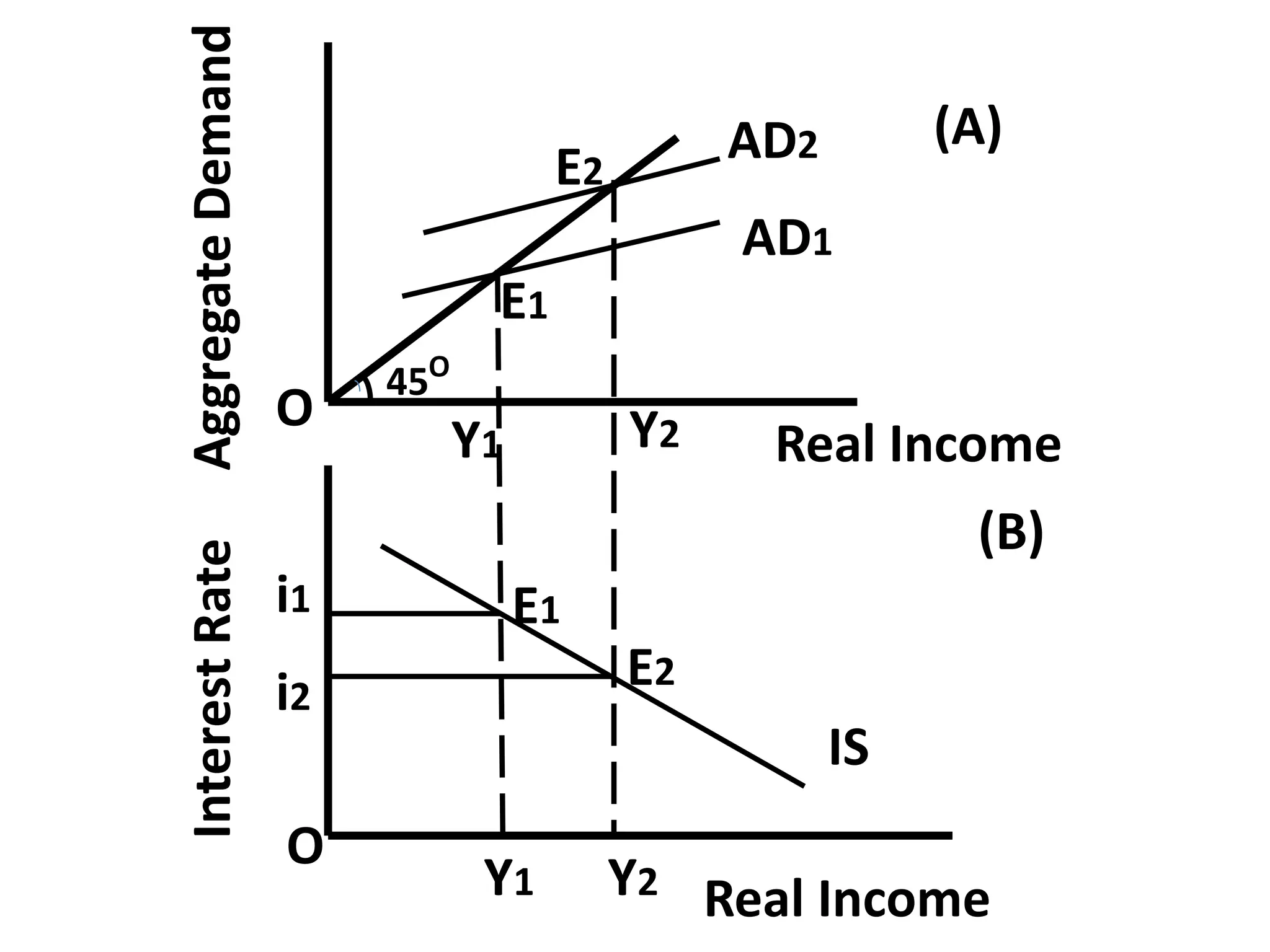
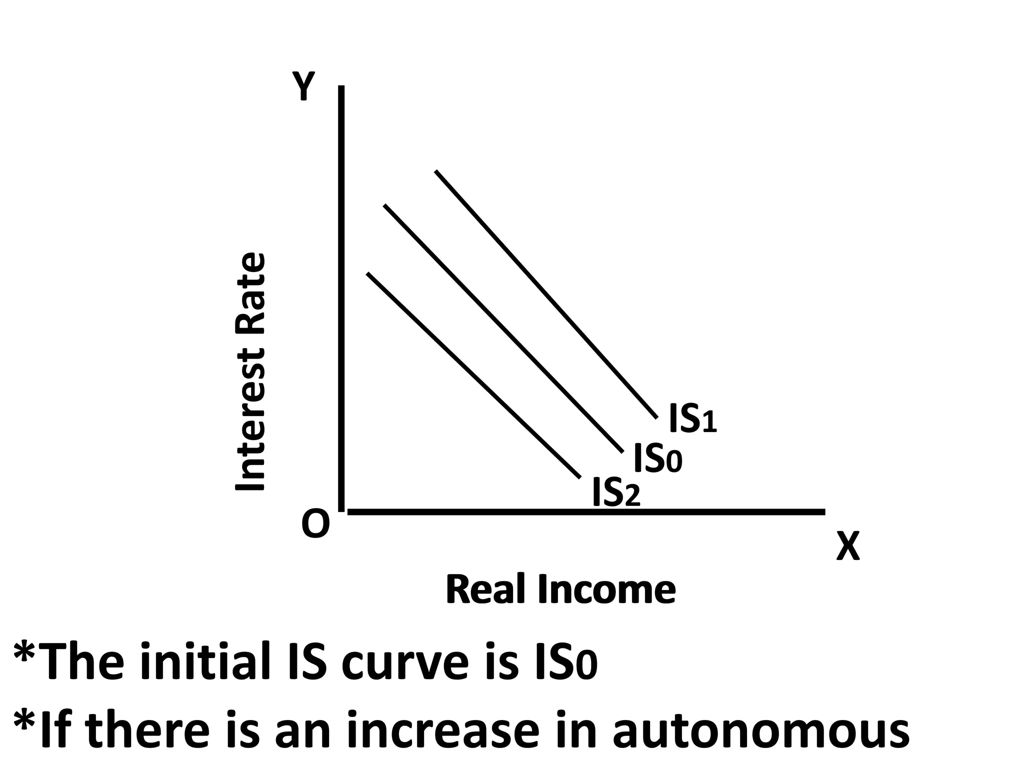
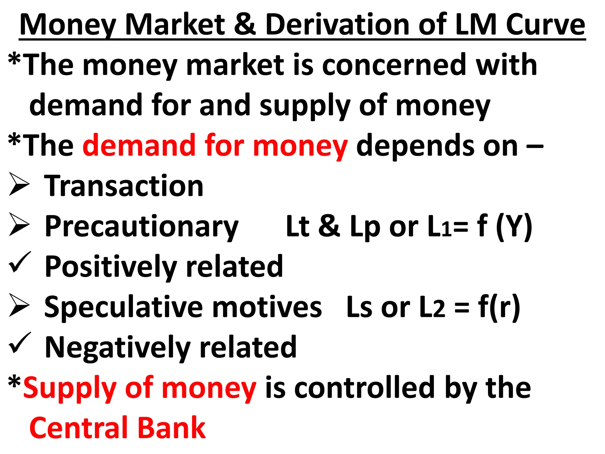
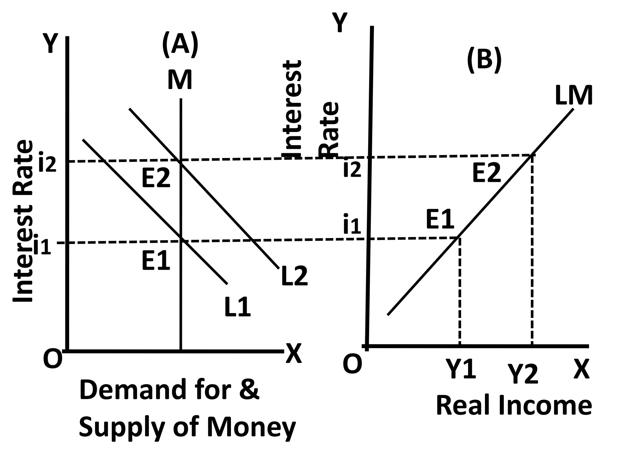
The IS-LM model shows the equilibrium in the goods market (IS curve) and money market (LM curve). The IS curve depicts combinations of interest rates and income levels where investment equals savings. It slopes downward because lower interest rates increase investment and shift aggregate demand outward, raising income. The LM curve shows combinations of interest rates and income where the demand for money equals the supply of money. It slopes upward because higher income increases money demand, shifting the demand curve right and raising the equilibrium interest rate. Together, the intersection of the IS and LM curves indicates the general equilibrium in the economy across both markets.

1. IS-LM Model
The Goods Market & the IS Curve
*The goods market is in equilibrium when
Output/ Income = Aggregate Demand
*At this point,
Saving = Investment
*Saving depends on the level of income
*It is directly related to income
*Investment depends on the rate of
interest
*It is inversely related to interest rate

2. *IS curve reflects the combination of the
interest rate & income
*So, Investment = Saving
I = S
*The goods market equilibrium is shown
by the IS curve
Derivation of IS Curve
*Diagram -

3. AD2
AD1
E1
E2
45O
Y1 Y2
IS
E1
E2
i2
i1
Y1 Y2
O
O
Real Income
Real Income
Aggregate
Demand
Aggregate
Demand
Interest
Rate
(A)
(B)

4. In this diagram-
*The given interest rate is - i1
*The aggregate demand curve AD1(part A)
intersects the 45 degree line at the point
E1
*It is an equilibrium point of goods
market
*Equilibrium income is Y1
*If the rate of interest falls to i2, aggregate
demand will rise
*The aggregate demand curve shifts

5. upwards to AD2
*The new equilibrium point is E2
*The equilibrium level of income rises to
Y2
*If we repeat this exercise for all
possible interest rates we can obtain a
series of combinations of interest rates
& levels of income at which the goods
market is in equilibrium
*By joining all these points in the B part of
Fig., we obtain the IS curve

6. *Thus, IS curve is the locus of pairs of
interest rates and levels of income
which are compatible with goods market
equilibrium
*The equilibrium is only on the IS curve
*Outside the IS curve, the goods market
is not in equilibrium
*Because at the right of the IS curve there
is excess supply in the goods market
*& the left of the IS curve there is excess
demand in the goods market

7. The Slope of IS Curve
*The IS curve slopes downwards
*Because a decrease in interest rate
increases investment
*Which shifts aggregate demand curve up
and rises the equilibrium income level
*The steepness of IS curve depends on the
sensitivity of investment spending and
autonomous consumption expenditure
to changes in interest rates
*If the investment spending and

8. autonomous consumption expenditure
are very sensitive to the interest rate,
then the change in interest rate will
produce a large change in aggregate
demand and it shows large change in
income level. In this case IS curve will
be flatter
*If the investment spending and
autonomous consumption expenditure
are not very sensitive to change in
interest rates then the IS curve will be

9. very steep
Shifts in IS Curve
*It is depend on –
1.Change in Govt. Spending –
 Increase in Govt. spending will shift the
IS curve to the right
 While a decrease in Govt. spending
shift the IS curve to the left
2.Change in Taxes –
 An increase in taxes will shift the IS
curve to the left

10.  While a decrease in taxes shift the IS
curve to the right
3.Autonomous Change in Investment –
 An increase in autonomous investment
will shift the IS curve to the right
 While a decrease in autonomous
investment will shift the IS curve to the
left
*Diagram -

11. IS1
IS0
IS2
O
Y
X
Real Income
Real Income
Interest
Rate
*The initial IS curve is IS0
*If there is an increase in autonomous

12. spending IS curve shifts right to IS1
*& if there is a fall in autonomous
spending IS curve shifts left to IS2

13. Money Market & Derivation of LM Curve
*The money market is concerned with
demand for and supply of money
*The demand for money depends on –
 Transaction
 Precautionary Lt & Lp or L1= f (Y)
 Positively related
 Speculative motives Ls or L2 = f(r)
 Negatively related
*Supply of money is controlled by the
Central Bank

14. *The money market is in equilibrium –
Demand for money = Supply of money
*The LM curve shows the combinations –
 Interest rate &
Income
*Diagram -

15. Y1
O
O X
Y
Y
X
E1
E2
i1
i2
i1
i2
LM
Y2
Interest
Rate
Real Income
Demand for &
Supply of Money
M
E2
E1
Interest
Rate
(B)
(A)
L1
L2

16. In this diagram –
*L1 is the original demand curve of money
*M is the original supply curve of money
*L1 & M interest each other at point E1
*At this equilibrium point (E1), the money
market is in equilibrium with the
combination of Y1 income and i1 interest
rate
*When income rises to Y2, the demand
curve shifts to L2
*The new equilibrium point is E2

17. *At this equilibrium point the money
market is in equilibrium with the
combination of Y2 income and i2 interest
rate
*In the (B) part of the diagram, we obtain
LM curve, by joining the equilibrium
points like E1 and E2
Slope of LM Curve
*The LM curve slopes upwards to the
right
*If the demand for money is relatively

18. insensitive to the interest rate, the LM
curve is close to vertical
*If the demand for money is very sensitive
to interest rate, the LM curve close to
horizontal