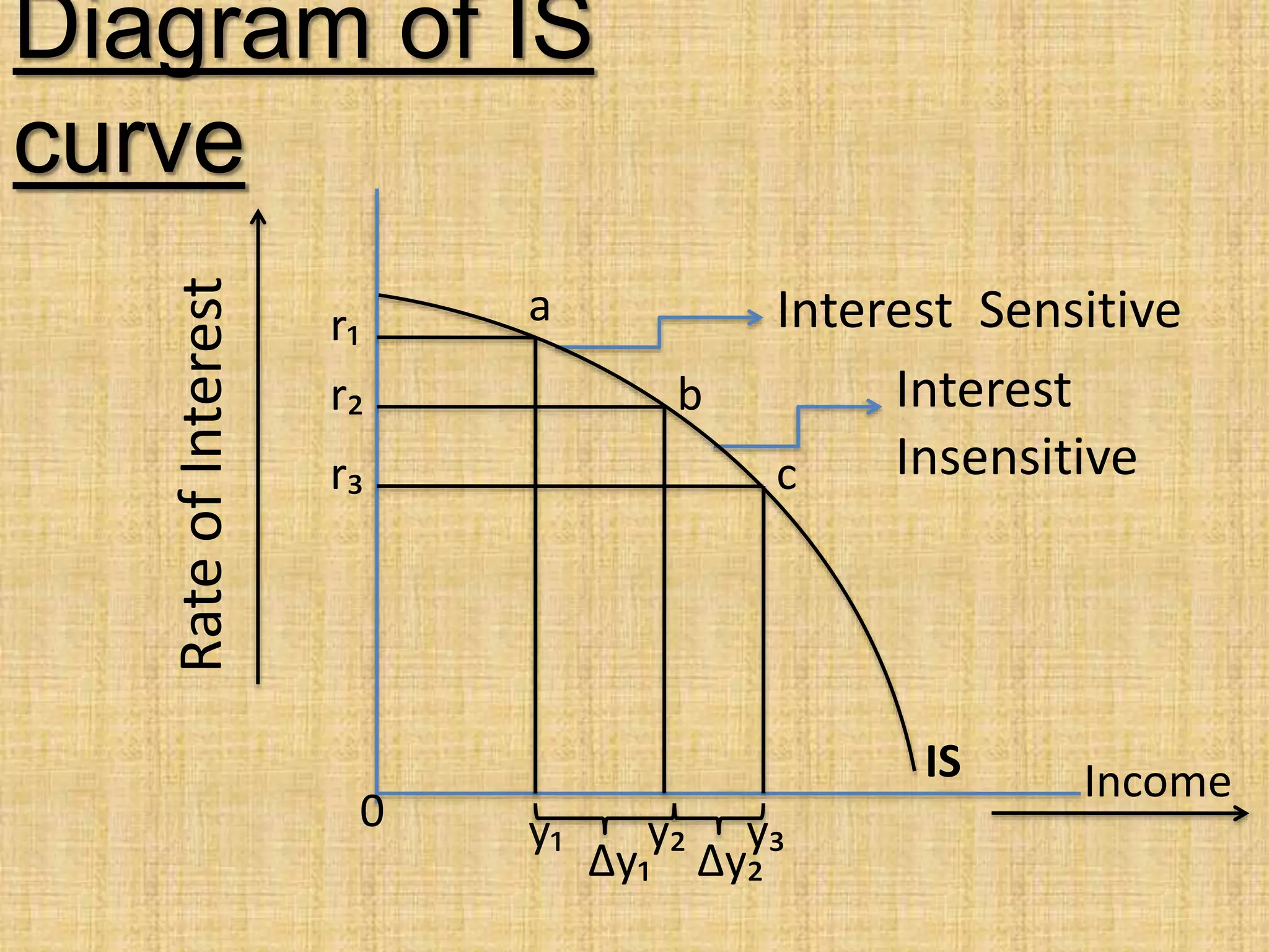
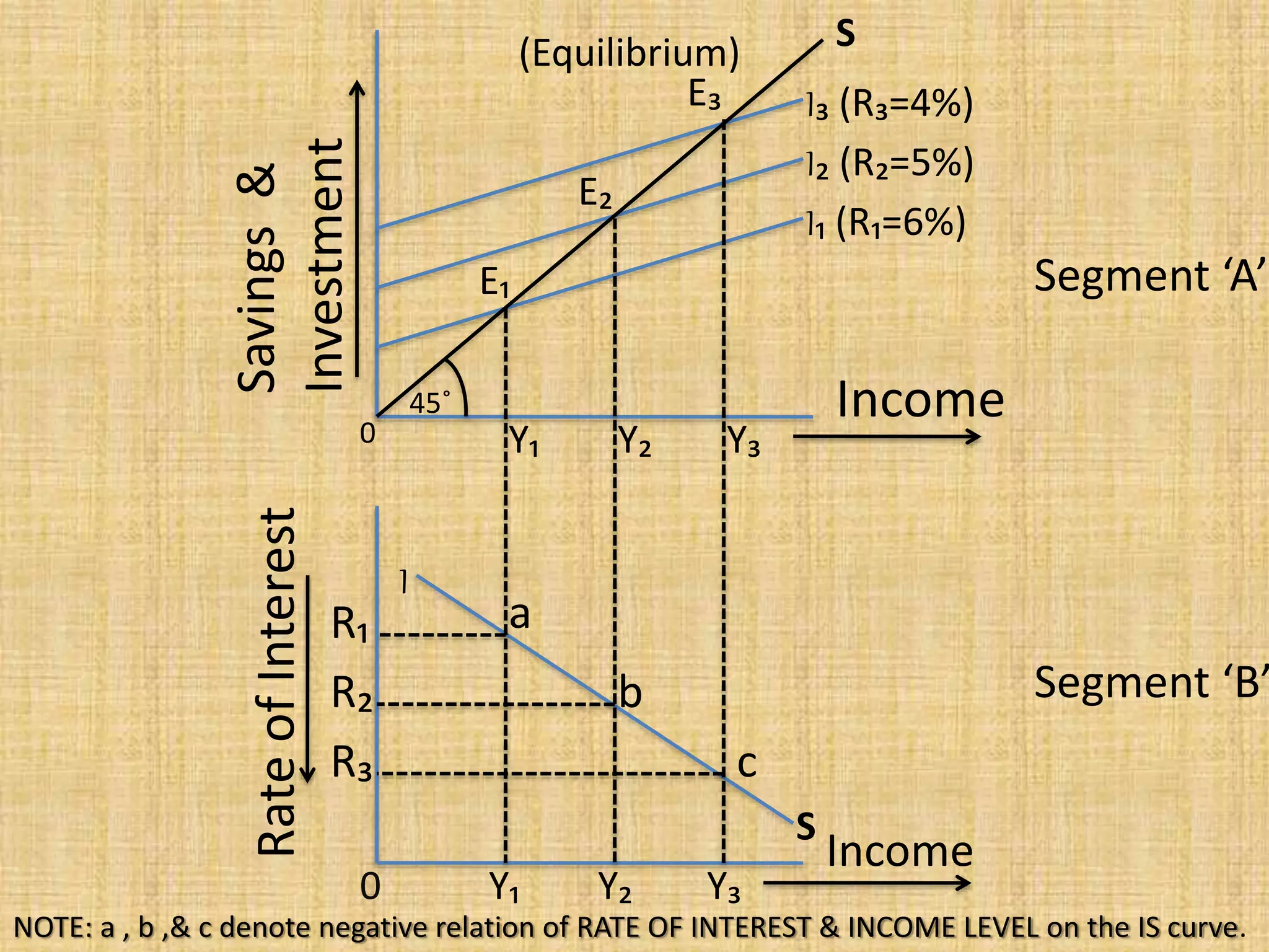
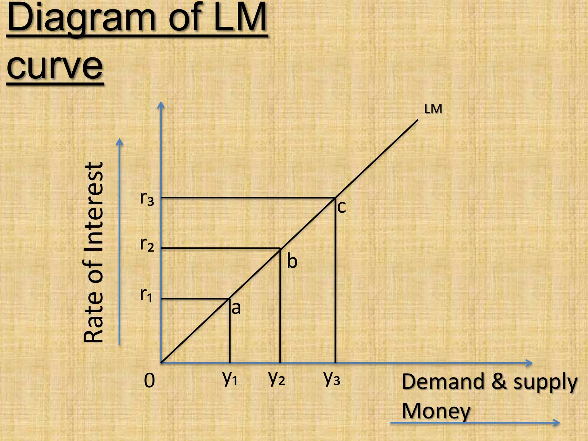
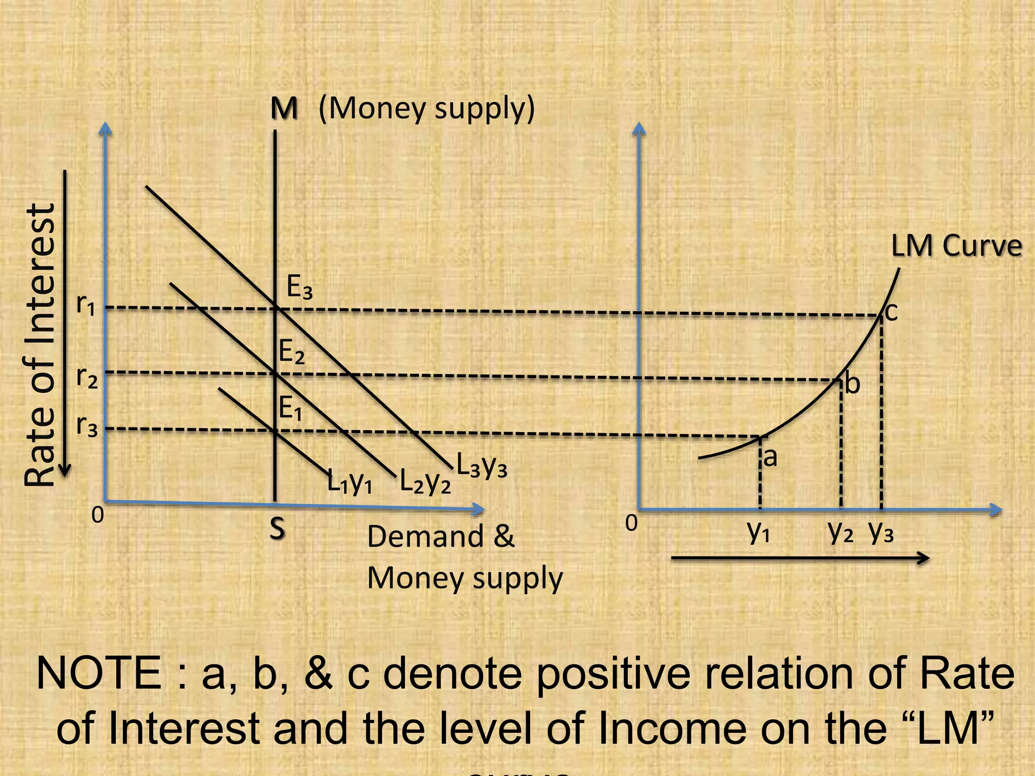
Basic Cncept Of “IS-
LM” Model
Presented by
“AMITIAN”
Amarjeet
Kumar
CONTENT
What is “IS-LM” model and some
features of “IS-LM”
model?
Slope of “IS” curve with suitable
diagram.
Negative relation of Rate of interest and
Income level on
the “IS” curve.
“IS-LM” MODEL
The “IS-LM” model translates the General
Theory of Keynes into neoclassical
terms(often called the neoclassical
synthesis).
It was proposed by John Hicks in 1937 in
a paper called “Mr Keynes.
The level of demand determines the level
of output and employment.
The “IS-LM” model is based on : The
investment-demand function, The
The model rests on two fundamental
assumption :
All prices (includes wages) are fixed.
There exist excess production capacity in
the economy.
The model examines the combined
equilibrium of two markets :
The goods market, which is at equilibrium
when investment equal saving, hence IS.
The money market, which is at equilibrium
SLOPE OF “IS” CURVE
‱Slope of “IS” given by impact of
change in interest rates on investment
and hence output (through multiplier) –
likely steep
‱Location of “IS” changed by
autonomous components of aggregate
demand ( e.g., autonomous investment,
r₁
r₂
r₃
a
b
c
IS Income
RateofInterest
0 y₁ y₃y₂
∆y₁ ∆y₂
Interest Sensitive
Interest
Insensitive
Diagram of IS
curve
S
E₃
E₂
E₁Savings&
Investment
Income
Y₁ Y₂ Y₃
I
S
R₁
R₂
R₃
0
0
RateofInterest
Y₁ Y₂ Y₃
Income
a
b
c
45˚
Segment ‘A’
Segment ‘B’
(Equilibrium)
I₃ (R₃=4%)
I₂ (R₂=5%)
I₁ (R₁=6%)
NOTE: a , b ,& c denote negative relation of RATE OF INTEREST & INCOME LEVEL on the IS curve.
SLOPE OF “LM”
CURVE
Slope of LM reflects interest and income
elasticity of money demand ( likely steep)
Location of LM : Expansionary Monetary
Policy raises real balances and hence
lowers interest rates at a giving level of real
income (LM curve shifts down and to right).
LM
Demand & supply
Money
RateofInterest
a
b
cr₃
r₂
r₁
0 y₁ y₂ y₃
Diagram of LM
curve
NOTE : a, b, & c denote positive relation of Rate
of Interest and the level of Income on the “LM”
M
S0 0 y₁ y₂ y₃
a
b
c
L₃y₃L₂y₂L₁y₁
E₃
E₂
E₁
r₁
r₂
r₃
(Money supply)
Demand &
Money supply
RateofInterest
M
S0 0
LM Curve
y₁ y₂ y₃
a
b
c
L₃y₃L₂y₂L₁y₁
E₃
E₂
E₁
r₁
r₂
r₃
(Money supply)
Demand &
Money supply
The End

Basic theory of IS-LM model

  • 1.
    Basic Cncept Of“IS- LM” Model Presented by “AMITIAN” Amarjeet Kumar
  • 2.
    CONTENT What is “IS-LM”model and some features of “IS-LM” model? Slope of “IS” curve with suitable diagram. Negative relation of Rate of interest and Income level on the “IS” curve.
  • 3.
    “IS-LM” MODEL The “IS-LM”model translates the General Theory of Keynes into neoclassical terms(often called the neoclassical synthesis). It was proposed by John Hicks in 1937 in a paper called “Mr Keynes. The level of demand determines the level of output and employment. The “IS-LM” model is based on : The investment-demand function, The
  • 4.
    The model restson two fundamental assumption : All prices (includes wages) are fixed. There exist excess production capacity in the economy. The model examines the combined equilibrium of two markets : The goods market, which is at equilibrium when investment equal saving, hence IS. The money market, which is at equilibrium
  • 5.
    SLOPE OF “IS”CURVE ‱Slope of “IS” given by impact of change in interest rates on investment and hence output (through multiplier) – likely steep ‱Location of “IS” changed by autonomous components of aggregate demand ( e.g., autonomous investment,
  • 6.
    r₁ r₂ r₃ a b c IS Income RateofInterest 0 y₁y₃y₂ ∆y₁ ∆y₂ Interest Sensitive Interest Insensitive Diagram of IS curve
  • 7.
    S E₃ E₂ E₁Savings& Investment Income Y₁ Y₂ Y₃ I S R₁ R₂ R₃ 0 0 RateofInterest Y₁Y₂ Y₃ Income a b c 45˚ Segment ‘A’ Segment ‘B’ (Equilibrium) I₃ (R₃=4%) I₂ (R₂=5%) I₁ (R₁=6%) NOTE: a , b ,& c denote negative relation of RATE OF INTEREST & INCOME LEVEL on the IS curve.
  • 8.
    SLOPE OF “LM” CURVE Slopeof LM reflects interest and income elasticity of money demand ( likely steep) Location of LM : Expansionary Monetary Policy raises real balances and hence lowers interest rates at a giving level of real income (LM curve shifts down and to right).
  • 9.
  • 10.
    NOTE : a,b, & c denote positive relation of Rate of Interest and the level of Income on the “LM” M S0 0 y₁ y₂ y₃ a b c L₃y₃L₂y₂L₁y₁ E₃ E₂ E₁ r₁ r₂ r₃ (Money supply) Demand & Money supply RateofInterest M S0 0 LM Curve y₁ y₂ y₃ a b c L₃y₃L₂y₂L₁y₁ E₃ E₂ E₁ r₁ r₂ r₃ (Money supply) Demand & Money supply
  • 11.