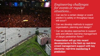
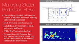
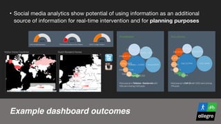
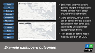
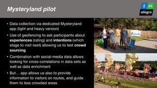
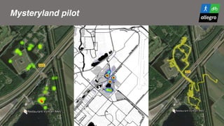
The document discusses the breakdown of efficient self-organization in pedestrian flows when density exceeds critical levels, leading to decreased flow performance and necessitating effective crowd management strategies. It highlights recent developments in real-time crowd management systems, including data collection at transportation hubs and event scenarios, as well as models for predicting pedestrian behavior and flow dynamics. The work explores integration of social media data with traditional monitoring for enhanced situational awareness and planning.

1. 1
Remember this?

2. 2
Break-down of efficient self-
organisation
• When conditions become too crowded
(density larger than critical density),
efficient self-organisation ‘breaks down’
• Flow performance (effective capacity)
decreases substantially, potentially causing
more problems as demand stays at same
level
• Importance of ‘keeping things flowing’, i.e.
keeping density at subcritical level
maintaining efficient and smooth flow
operations
• Has severe implications on the network level

3. Why crowd management is necessary!
• Pedestrian Network Fundamental Diagram
shows relation between number of
pedestrians in area
• P-NFD shows reduced performance of
network flow operations in case of
overloading causes by various phenomena
such as faster-is-slower effect and self-
organisation breaking down
• Current work focusses on theory P-NFD,
hysteresis, and impact of spatial variation
(forthcoming ISTTT paper)
Qnetwork(⇢, ) = Qlocal(⇢)
v0
⇢jam
2

4. ITS For Crowds
Intelligent Crowd Management
Prof. dr. Serge Hoogendoorn
4

5. 5
Engineering challenges
for events or regular
situations…
• Can we for a certain design or event
predict if a safety or throughput issue
will occur?
• Can we develop methods to support
organisation, planning and design?
• Can we develop approaches to support
safe and efficient real-time management
of (large) pedestrian flows?
Presentation will go into recent
developments in the field op real-time
crowd management support with key
elements: real-time monitoring &
prediction

6. WiFi/BT data on Utrecht Central Station
Managing Station
Pedestrian Flows
• Dutch railway (ProRail and NS) with
support of TU Delft have been working
on SmartStation concept
• Multi-level data collection system
• Detailed density collection at pinch
points (e.g. platforms)
• WiFi / BlueTooth at station level
• Combination with Chipcard data
provides comprehensive monitoring
information for ex-post assessment
and real-time interventions
Trajectory data from one of the platforms

7. 7
Monitoring and predicting active
traffic in cities (for regular and
event conditions)
• Unique pilots with crowd management system
for large scale, outdoor event
• Functional architecture of SAIL 2015 crowd
management systems, also used for Europride,
Mysteryland, Kingsday
• Phase 1 focussed on monitoring and
diagnostics (data collection, number of visitors,
densities, walking speeds, determining levels of
service and potentially dangerous situations)
• Phase 2 focusses on prediction and decision
support for crowd management measure
deployment (model-based prediction,
intervention decision support)
Data
fusion and
state estimation:
hoe many people
are there and how
fast do they
move?
Social-media
analyser: who are
the visitors and what
are they talking
about?
Bottleneck
inspector: wat
are potential
problem
locations?
State
predictor: what
will the situation
look like in 15
minutes?
Route
estimator:
which routes
are people
using?
Activity
estimator:
what are
people
doing?
Intervening:
do we need to
apply certain
measures and
how?

8. Example of
tracking data
collected during
SAIL 2015
Additional data fro
counting cameras,
Wifi trackers, etc.,
provide
comprehensive
real-time picture of
situation during
event
Plans to use this as
a basis for the
Amsterdam Smart
Tourist dashboard

9. Example dashboard outcomes
• Newly developed algorithm to distinguish between
occupancy time and walking time
• Other examples show volumes and OD flows
• Results used for real-time intervention, but also for
planning of SAIL 2020 (simulation studies)
0
5
10
15
20
25
30
11 12 13 14 15 16 17 18 19
verblijftijd looptijd
1988
1881
4760
4958
2202
1435
6172
59994765
4761
4508
3806
3315
2509
1752
3774
4061
2629
1359
2654
2139
1211
1439
2209
1638
2581
31102465
3067
2760

10. Example dashboard outcomes
• Social media analytics show potential of using information as an additional
source of information for real-time intervention and for planning purposes

11. Example dashboard outcomes
• Sentiment analysis allows
gaining insight into locations
where people tweet about
crowdedness conditions
• More generally, focus is on
use of social (media) data (in
conjunction with other data
sources) to unravel urban
transportation flows
• First phase of active mode
mobility lab (part of UML)
Druk
Vol
Gedrang
Bomvol
Boordevol
Afgeladen
Volgepakt
Crowded
Busy
Jam
Jam-
Buitenlandse toeristen
Inwoners Amsterdam

12. Social media data based count reproduction
• Is it possible to
reconstruct counts from
social-media data?
• Compare different
methods to see which
represents measurements
of density using WiFi/BT
• Time-space averaging
provides poor results
• Speed and flow based
methods look very
promising!
12

13. Mysteryland pilot
• Data collection via dedicated Mysteryland
app (light and heavy version)
• Use of geofencing to ask participants about
experiences (rating) and intentions (which
stage to visit next) allowing us to test crowd
sourcing
• Combination with social-media data allows
looking for cross-correlations in data sets as
well as data enrichment
• But… app allows us also to provide
information to visitors on routes, and guide
them to less crowded areas 13

14. e: mysteryland music festival
Mysteryland pilot
14

15. Modelling for planning
Application of differential game theory:
• Pedestrians minimise predicted walking cost, due
to straying from intended path, being too close to
others / obstacles and effort, yielding:
• Simplified model is similar to Social Forces model of Helbing
Face validity?
• Model results in reasonable macroscopic flow characteristics (capacity
values and fundamental diagram)
• What about self-organisation?
15
1. Introduction
This memo aims at connecting the microscopic modelling principles underlying the
social-forces model to identify a macroscopic flow model capturing interactions amongst
pedestrians. To this end, we use the anisotropic version of the social-forces model pre-
sented by Helbing to derive equilibrium relations for the speed and the direction, given
the desired walking speed and direction, and the speed and direction changes due to
interactions.
2. Microscopic foundations
We start with the anisotropic model of Helbing that describes the acceleration of
pedestrian i as influence by opponents j:
(1) ~ai =
~v0
i ~vi
⌧i
Ai
X
j
exp

Rij
Bi
· ~nij ·
✓
i + (1 i)
1 + cos ij
2
◆
where Rij denotes the distance between pedestrians i and j, ~nij the unit vector pointing
from pedestrian i to j; ij denotes the angle between the direction of i and the postion
of j; ~vi denotes the velocity. The other terms are all parameters of the model, that will
be introduced later.
In assuming equilibrium conditions, we generally have ~ai = 0. The speed / direction
for which this occurs is given by:
(2) ~vi = ~v0
i ⌧iAi
X
j
exp

Rij
Bi
· ~nij ·
✓
i + (1 i)
1 + cos ij
2
◆
Let us now make the transition to macroscopic interaction modelling. Let ⇢(t, ~x)
Level of anisotropy
reflected by this
parameter
~vi
~v0
i
~ai
~nij
~xi
~xj

16. • Simple model shows plausible self-
organised phenomena
• Model also shows flow breakdown
in case of overloading
• Similar model has been
successfully used for planning of
SAIL, but it is questionable if for
real-time purposes such a model
would be useful, e.g. due to
complexity
• Coarser models proposed so far
turn out to have limited predictive
validity, and are unable to
reproduce self-organised patterns
• Develop continuum model based on
game-theoretical model NOMAD…
Microscopic models aretoo computationallycomplex for real-timeapplication and lack niceanalytical properties…

17. Modelling for real-time predictions
• NOMAD / Social-forces model as starting point:
• Equilibrium relation stemming from model (ai = 0):
• Interpret density as the ‘probability’ of a pedestrian being present, which gives a macroscopic equilibrium
relation (expected velocity), which equals:
• Combine with conservation of pedestrian equation yields complete model, but numerical integration is
computationally very demanding
17
sented by Helbing to derive equilibrium relations for the speed and the direction, given
the desired walking speed and direction, and the speed and direction changes due to
interactions.
2. Microscopic foundations
We start with the anisotropic model of Helbing that describes the acceleration of
pedestrian i as influence by opponents j:
(1) ~ai =
~v0
i ~vi
⌧i
Ai
X
j
exp

Rij
Bi
· ~nij ·
✓
i + (1 i)
1 + cos ij
2
◆
where Rij denotes the distance between pedestrians i and j, ~nij the unit vector pointing
from pedestrian i to j; ij denotes the angle between the direction of i and the postion
of j; ~vi denotes the velocity. The other terms are all parameters of the model, that will
be introduced later.
In assuming equilibrium conditions, we generally have ~ai = 0. The speed / direction
for which this occurs is given by:
(2) ~vi = ~v0
i ⌧iAi
X
j
exp

Rij
Bi
· ~nij ·
✓
i + (1 i)
1 + cos ij
2
◆
Let us now make the transition to macroscopic interaction modelling. Let ⇢(t, ~x)
denote the density, to be interpreted as the probability that a pedestrian is present on
location ~x at time instant t. Let us assume that all parameters are the same for all
pedestrian in the flow, e.g. ⌧i = ⌧. We then get:
(3) ZZ ✓
||~y ~x||
◆ ✓
1 + cos xy(~v)
◆
~y ~x
We start with the anisotropic model of Helbing that describes the acceleration of
pedestrian i as influence by opponents j:
(1) ~ai =
~v0
i ~vi
⌧i
Ai
X
j
exp

Rij
Bi
· ~nij ·
✓
i + (1 i)
1 + cos ij
2
◆
where Rij denotes the distance between pedestrians i and j, ~nij the unit vector pointing
from pedestrian i to j; ij denotes the angle between the direction of i and the postion
of j; ~vi denotes the velocity. The other terms are all parameters of the model, that will
be introduced later.
In assuming equilibrium conditions, we generally have ~ai = 0. The speed / direction
for which this occurs is given by:
(2) ~vi = ~v0
i ⌧iAi
X
j
exp

Rij
Bi
· ~nij ·
✓
i + (1 i)
1 + cos ij
2
◆
Let us now make the transition to macroscopic interaction modelling. Let ⇢(t, ~x)
denote the density, to be interpreted as the probability that a pedestrian is present on
location ~x at time instant t. Let us assume that all parameters are the same for all
pedestrian in the flow, e.g. ⌧i = ⌧. We then get:
(3)
~v = ~v0
(~x) ⌧A
ZZ
~y2⌦(~x)
exp
✓
||~y ~x||
B
◆ ✓
+ (1 )
1 + cos xy(~v)
2
◆
~y ~x
||~y ~x||
⇢(t, ~y)d~y
Here, ⌦(~x) denotes the area around the considered point ~x for which we determine the
interactions. Note that:
pedestrian i as influence by opponents j:
(1) ~ai =
~v0
i ~vi
⌧i
Ai
X
j
exp

Rij
Bi
· ~nij ·
✓
i + (1 i)
1 + cos ij
2
◆
where Rij denotes the distance between pedestrians i and j, ~nij the unit vector pointing
from pedestrian i to j; ij denotes the angle between the direction of i and the postion
of j; ~vi denotes the velocity. The other terms are all parameters of the model, that will
be introduced later.
In assuming equilibrium conditions, we generally have ~ai = 0. The speed / direction
for which this occurs is given by:
(2) ~vi = ~v0
i ⌧iAi
X
j
exp

Rij
Bi
· ~nij ·
✓
i + (1 i)
1 + cos ij
2
◆
Let us now make the transition to macroscopic interaction modelling. Let ⇢(t, ~x)
denote the density, to be interpreted as the probability that a pedestrian is present on
location ~x at time instant t. Let us assume that all parameters are the same for all
pedestrian in the flow, e.g. ⌧i = ⌧. We then get:
(3)
~v = ~v0
(~x) ⌧A
ZZ
~y2⌦(~x)
exp
✓
||~y ~x||
B
◆ ✓
+ (1 )
1 + cos xy(~v)
2
◆
~y ~x
||~y ~x||
⇢(t, ~y)d~y
Here, ⌦(~x) denotes the area around the considered point ~x for which we determine the
interactions. Note that:
(4) cos xy(~v) =
~v
||~v||
·
~y ~x
||~y ~x||

18. Modelling for real-time predictions
• Taylor series approximation:
yields a closed-form expression for the equilibrium velocity , which is given by the equilibrium
speed and direction:
with:
• Check behaviour of model by looking at isotropic flow ( ) and homogeneous flow
conditions ( )
• Include conservation of pedestrian relation gives a complete model…
18
2 SERGE P. HOOGENDOORN
From this expression, we can find both the equilibrium speed and the equilibrium direc-
tion, which in turn can be used in the macroscopic model.
We can think of approximating this expression, by using the following linear approx-
imation of the density around ~x:
(5) ⇢(t, ~y) = ⇢(t, ~x) + (~y ~x) · r⇢(t, ~x) + O(||~y ~x||2
)
Using this expression into Eq. (3) yields:
(6) ~v = ~v0
(~x) ~↵(~v)⇢(t, ~x) (~v)r⇢(t, ~x)
with ↵(~v) and (~v) defined respectively by:
(7) ~↵(~v) = ⌧A
ZZ
~y2⌦(~x)
exp
✓
||~y ~x||
B
◆ ✓
+ (1 )
1 + cos xy(~v)
2
◆
~y ~x
||~y ~x||
d~y
and
(8) (~v) = ⌧A
ZZ
~y2⌦(~x)
exp
✓
||~y ~x||
B
◆ ✓
+ (1 )
1 + cos xy(~v)
2
◆
||~y ~x||d~y
To investigate the behaviour of these integrals, we have numerically approximated
FROM MICROSCOPIC TO MACROSCOPIC INTERACTION MODELING 3
Furthermore, we see that for ~↵, we find:
(10) ~↵(~v) = ↵0 ·
~v
||~v||
(Can we determine this directly from the integrals?)
From Eq. (6), with ~v = ~e · V we can derive:
(11) V = ||~v0
0 · r⇢|| ↵0⇢
and
(12) ~e =
~v0
0 · r⇢
V + ↵0⇢
=
~v0
0 · r⇢
||~v0
0 · r⇢||
Note that the direction does not depend on ↵0, which implies that the magnitude of
the density itself has no e↵ect on the direction, while the gradient of the density does
influence the direction.
2.1. Homogeneous flow conditions. Note that in case of homogeneous conditions,
FROM MICROSCOPIC TO MACROSCOPIC INTERACTION MODELING 3
Furthermore, we see that for ~↵, we find:
(10) ~↵(~v) = ↵0 ·
~v
||~v||
(Can we determine this directly from the integrals?)
From Eq. (6), with ~v = ~e · V we can derive:
(11) V = ||~v0
0 · r⇢|| ↵0⇢
and
(12) ~e =
~v0
0 · r⇢
V + ↵0⇢
=
~v0
0 · r⇢
||~v0
0 · r⇢||
Note that the direction does not depend on ↵0, which implies that the magnitude of
the density itself has no e↵ect on the direction, while the gradient of the density does
influence the direction.
2.1. Homogeneous flow conditions. Note that in case of homogeneous conditions,
i.e. r⇢ = ~0, Eq. (11) simplifies to
(13) V = ||~v0|| ↵0⇢ = V 0
↵0⇢
α0 = πτ AB2
(1− λ) and β0 = 2πτ AB3
(1+ λ)
4.1. Analysis of model properties
Let us first take a look at expressions (14) and (15) describing the equilibrium290
speed and direction. Notice first that the direction does not depend on ↵0, which
implies that the magnitude of the density itself has no e↵ect, and that only the
gradient of the density does influence the direction. We will now discuss some
other properties, first by considering a homogeneous flow (r⇢ = ~0), and then
by considering an isotropic flow ( = 1) and an anisotropic flow ( = 0).295
4.1.1. Homogeneous flow conditions
Note that in case of homogeneous conditions, i.e. r⇢ = ~0, Eq. (14) simplifies
sions (14) and (15) describing the equilibrium
at the direction does not depend on ↵0, which
density itself has no e↵ect, and that only the
nce the direction. We will now discuss some
ng a homogeneous flow (r⇢ = ~0), and then
= 1) and an anisotropic flow ( = 0).
ns
us conditions, i.e. r⇢ = ~0, Eq. (14) simplifies
↵0⇢ = V 0
↵0⇢ (16)
!
v =
!
e ⋅V

19. 19
Macroscopic model
yields plausible
results…
• First macroscopic model able to
reproduce self-organised patterns
(lane formation, diagonal stripes)
• Self-organisation breaks downs in
case of overloading
• Continuum model seems to
inherit properties of the
microscopic model underlying it
• Forms solid basis for real-time
prediction module in dashboard
• First trials in model-based
optimisation and use of model for
state-estimation are promising

20. Predicting flow operations in Laussanne
• Work performed by Flurin
Haenseler showing how
LOS can be predicted by
using macroscopic model
• Example shows LOS in one
of the corridors connecting
platforms in the station
• Flow model + route choice
model used for Origin-
Destination matrix
estimation using counts
and time-table information

21. Towards active interventions
• Models can be used to improve design
• Off-line model-based optimisation of signage /
evacuation instructions (see example)
• Crowd Monitoring Dashboard Amsterdam has been used
by crowd managers for real-time changes in circulation
plan (making some of the routes uni-directional)
• Other measures (in particular in stations) include load
balancing (changing time table, stop position of train,
track assignment), but also gating application
• Current research focusses on these type of interventions
21
x−axis (m)
y−axis(m)
Densities at t = 25.1 s
5 10 15 20 25 30 35 40 45 50
5
10
15
20
25
30
35
40
45
50
0
0.5
1
1.5
2
2.5
3
3.5
4
4.5
5
y−axis(m)
1
1
2
2
3
3
4
4
5
x−axis (m)
y−axis(m)
Densities at t = 50.1 s
5 10 15 20 25 30 35 40 45 50
5
10
15
20
25
30
35
40
45
50
0
0.5
1
1.5
2
2.5
3
3.5
4
4.5
5
x−axis (m)
y−axis(m)
Densities at t = 125.1 s
5 10 15 20 25 30 35 40 45 50
5
10
15
20
25
30
35
40
45
50
0
0.5
1
1.5
2
2.5
3
3.5
4
4.5
5
No redistribution of
queues (initial iteration)
x−axis (m)
y−axis(m)
Densities at t = 25.1 s
5 10 15 20 25 30 35 40 45 50
5
10
15
20
25
30
35
40
45
50
0
0.5
1
1.5
2
2.5
3
3.5
4
4.5
5
x−axis (m)
y−axis(m)
Densities at t = 125.1 s
5 10 15 20 25 30 35 40 45 50
5
10
15
20
25
30
35
40
45
50
0
0.5
1
1.5
2
2.5
3
3.5
4
4.5
5
x−axis (m)
y−axis(m)
Densities at t = 50.1 s
5 10 15 20 25 30 35 40 45 50
5
10
15
20
25
30
35
40
45
50
0
0.5
1
1.5
2
2.5
3
3.5
4
4.5
5
x−axis (m)
y−axis(m)
Densities at t = 125.1 s
5 10 15 20 25 30 35 40 45 50
5
10
15
20
25
30
35
40
45
50
0
0.5
1
1.5
2
2.5
3
3.5
4
4.5
5
No redistribution of
queues (initial iteration)
Distribution of queues
considering reduced speeds

22. Recall the P-MFD?
Ensuring that the number of pedestrians in
a railway stations states below critical level
by means of gating…

23. The ALLEGRO programme
unrAvelLing sLow modE travelinG and tRaffic:
with innOvative data to a new transportation and traffic theory for
pedestrians and bicycles”
• 4.1 million AUD personal grant with a focus on developing theory (from an
application oriented perspective) sponsored by the ERC and AMS
• Relevant elements of the project:
• Development of “living” data & simulation laboratory building on two decades of experience in
pedestrian monitoring, theory and simulation
• Outreach to cities by means of “solution-oriented” projects (“the AMS part”), e.g. event planning
framework, design and crowd management strategies, active mode operations dashboard, etc.
• Team is complete (9 PhD and 4 PD + 8 supervisors / support staff )

24. 25
Questions?