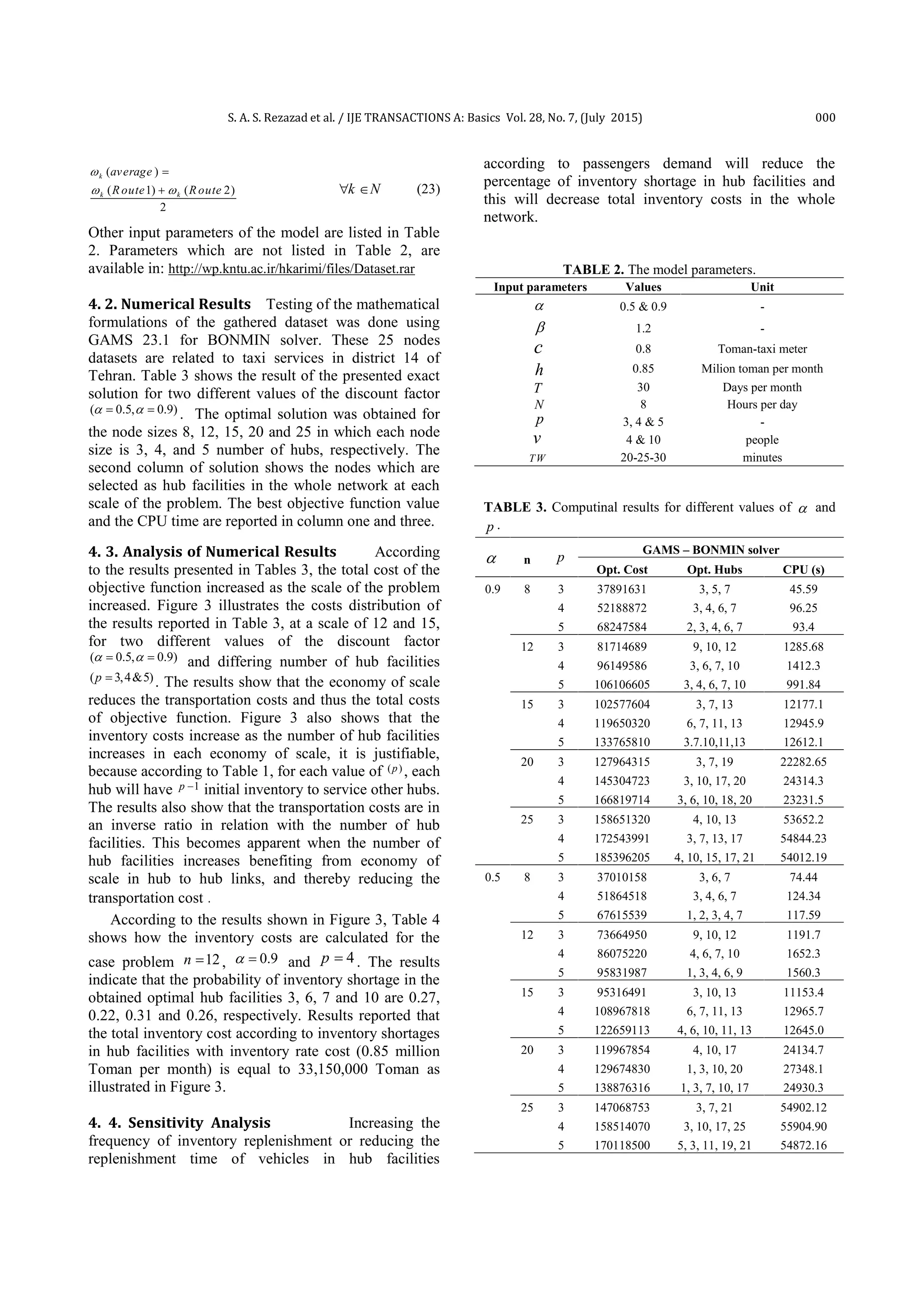
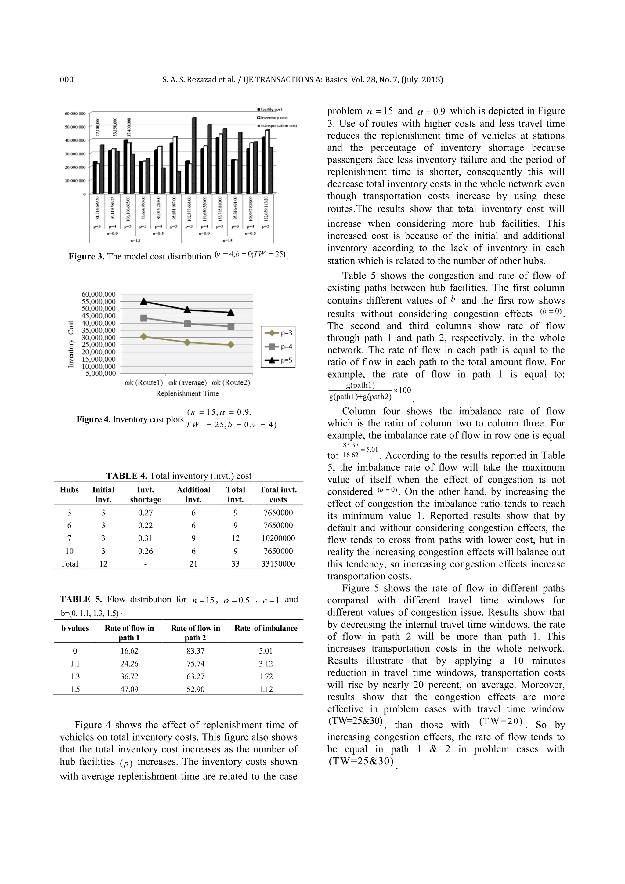
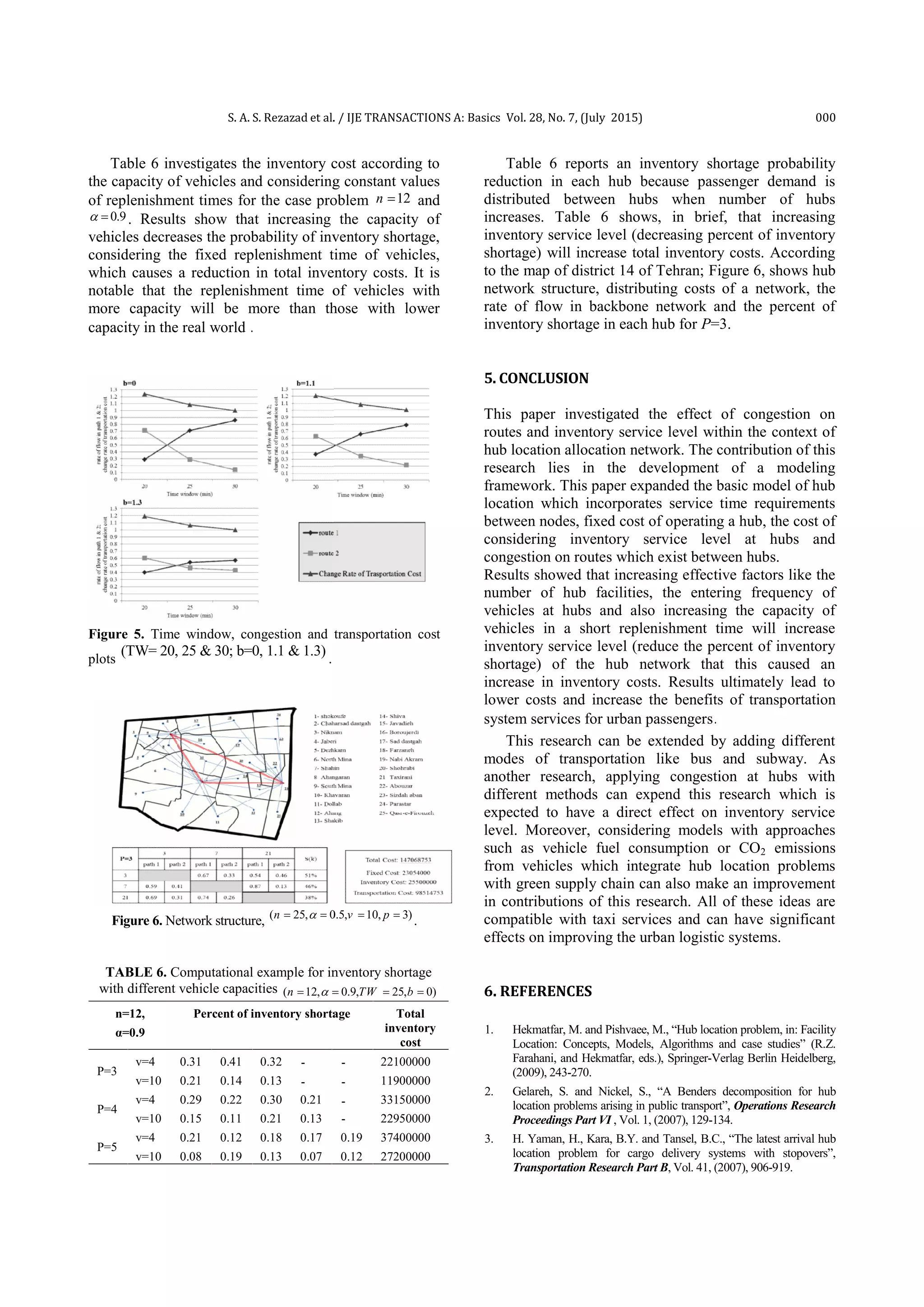
SlideShare a Scribd company logo
Please cite this article as: S. A. S. Rezazad, M. Aminnayeri, H. Karimi, A Congested Double Path Approach for a Hub Location-allocation Problem
with Service Level at Hubs, International Journal of Engineering (IJE), IJE TRANSACTIONS A: Basics Vol. 28, No. 7, (July 2015) ……
International Journal of Engineering
J o u r n a l H o m e p a g e : w w w . i j e . i r
A Congested Double Path Approach for a Hub Location-allocation Problem with
Service Level at Hubs
S. A. S. Rezazad* a, M. Aminnayeria, H. Karimi b
a Department of Industrial Engineering and Management Systems, Amir Kabir University of Technology, Iran.
b Department of Industrial Engineering, K.N.Toosi University of Technology, Iran
P A P E R I N F O
Paper history:
Received 25 December 2014
Received in revised form 28 March 2015
Accepted 11 June 2015
Keywords:
Hub Location Allocation
Inventory Service Level
Congestion
Double Path Approach
A B S T R A C T
In this paper an uncapacitated multiple allocation p-hub median problem is discussed. The model
minimizes the transportation cost based on inventory service level at hubs through double paths between
hubs. Inventory service level is defined as the percent of inventory shortage of vehicles at hubs according
to passengers demand and replenishment time of vehicles. A real data from 25 nodes of municipality
district 14 of Tehran is used to evaluate the performance of inventory service level in hub networks.
doi: 10.5829/idosi.ije.2015.28.07a.00.
Sets: k Replenishment time of vehicles at hub k.
N Set of all nodes indexed by i or j. ikt Time of transit from origin i to origin hub k.
,K l Origin and destination hub nodes, respectively. kmlt Time of transit from hub k to hub l via route m.
M Set of paths between hubs in whole network indexed by m. ljt Time of transit from destination hub l to destination j.
Parameters: kF Fixed cost of opening a hub at node k.
ijW The yearly flows from origin i to destination j. ijTW Service time window from node i to node j.
ikd Distance from origin i to origin hub k. Variables:
kmld Distance from origin hub k to destination hub l via route m.
ikmljX Equals one if flow from i to j is assigned to hub pair (k,l)
and route m and otherwise 0.ljd Distance from destination hub l to destination j.
ikc Unit transportation cost from origin i to origin hub k. kH Equals one if node k is a hub and otherwise 0.
kmlc Unit transportation cost from origin hub k to destination hub l via route m.
kS Probability of inventory shortage at hub k.
ljc Unit transportation cost from destination hub l to destination j.
 Cost discount factor 0 1  (applied for hub links). mg
Total flow in each kind of routes in hub links in whole
network.
 Time delay factor 1  (applied for hub links).
1. INTRODUCTION1
In recent years much researches in design and
performance of transportation systems have been carried
out to investigate the least expensive methods. There are
*Corresponding Author’s Email: a.s.rezazad@aut.ac.ir (S. A. S.
Rezazad)
two kinds of transportation systems: direct sending and
hub network. In direct systems, flow from origin to
destination will be sent directly and without considering
other destinations. So every vehicle in each trip is faced
with only one destination. This system is used
especially when the volume of cargo is large or it is
customize. On the other hand, when direct
communication between the origin and destination in a
IJE TRANSACTIONS A: Basics Vol. 28, No. 7, (July 2015)
S. A. S. Rezazad et al. / IJE TRANSACTIONS A: Basics Vol. 28, No. 7, (July 2015) 000
network is impossible or too costly, the second type of
system, the hub network is used. In this system the
flows are collected in a point which is called hub, and
then distributed between destinations. So in designing of
hub networks, strategic decision making like locating
hubs and assigning points of origins and destinations
should be adopted. Hub networks have the advantage
that the size of the vehicles will be determined by
economy, thus the economic benefits from the use of
vehicles and service level will be improved in this
system [1].
Taxi service is one of the applications of hub
location allocation problems. There are a lot of
terminals within the urban logistic network and paths
between each pair of origins and destinations should be
determined in such way that passengers reach their final
destination with the lowest cost and within a certain
time period. Public transportation were investigated in
hub location problems by Gelare and Nickel [2] and
Yaman et al. [3]. Moreover, an integrated incomplete
hub location-routing network is recently investigated by
Karimi and Setak [4], in a similar research. One of the
main applications of their model is the transportation
system, specially public and urban transportation.
Increased traffic and congestion in some routes
(especially connections between hub facilities), are
factors which may cause pauses and a lot of problems in
urban logistic systems. Because the volumes of daily
travel between hub facilities are greater than those
between other points in the network, this may cause
some disorders in urban transportation systems. In such
circumstances, using alternative paths to send flows
between hubs will improve the performance of the
network [5]. In this paper, a hub location allocation
problem for an urban logistic system is investigated
which contains two kinds of paths between hubs that
differ in terms of travel time and expense, such that
routes with a lower cost yield more travel time and vice
versa. Additionally, this paper also considers the
inventory service level at hubs and congestion on routes
between hub facilities in the whole network. The
contributions will be helpful in designating hub
networks with minimum vehicles at hubs to give good
services. According to congestion, this part of
contribution can be helpful to balance and manage
existing alternative paths between hub nodes and this is
helpfully applicable for limited zone by using traffic
cameras or some other related tools to control traffic in
real world. All of these applications are considered in
this work.
The rest of this paper is organized as follows:
section 2 presents and identifies the contribution of
relevant prior researches. The third section describes a
mixed integer nonlinear mathematical model.
Computational results and sensitivity analysis are
presented in section 4 and lastly, conclusions and
further research directions are discussed in section 5.
2. LITERATURE REVIEW
The literature related to this research can be found in
these main areas: p-hub median problems, hub problems
under congestion at hubs and location problems
considering inventory cost using the (S, S-1). The
mentioned areas are discussed below:
2. 1. pHMP Literature Although a variety of
models have been developed and investigated in the
context of hub related problems, they can be assigned to
the following main classes: the hub covering location
problem (HCLP) [6], the p-hub center problem (pHCP)
[6] and the p-hub median problem (pHMP) which is
related to this research. In a pHMP, the objective is to
locate “p” hubs in the network so that the total costs of
transporting flows through the network are minimized
[7]. Campbell [6] proposed pHCP based on the Mini-
Max criterion by which the maximum transportation
cost between all origin and destination pairs is
minimized. This type of problem is useful for
emergency facility locations. He also defined HCLP to
locate hubs in a way that each none-hub node is covered
by a pair of hub nodes. Karimi and Bashiri [8] presented
an adequate literature review of this problem and
developed a model with different coverage types.
There are two kinds of allocations: single and
multiple. In single allocation hub location problems,
each none-hub node is allocated to exactly one hub [9]
and in multiple allocations a none-hub node can be
allocated to more than one hub [10]. In this paper the
multiple allocation version of the p-hub median problem
is considered. The hub location problem was first
presented with a quadratic integer formulation by
O’Kelly [11]. He also proved that this is a NP-hard
problem. Klincewicz [12] presented two heuristics, one
based on exchanges of spoke assignments and the other
one based on clustering nodes. He also proposed the
tabu search and greedy randomized heuristic search.
Campbell [7] for the first time formulated pHMP with
multiple allocations as an integer programming model.
He also formulated an integer programming model
considering the threshold flow [13]. Skorin Kapov and
Skorin Kapov [14] presented a tabu search heuristic to
solve pHMP. Skorin Kapov et al. [15] formulated a
mixed integer pHMP and used an exact solution to solve
presented model. Ernest and Krishnamoorty [16]
proposed a linear programming formulation to solve the
pHMP and used simulated annealing to reach the upper
bound for the LP based branch and bound. Smith et al.
[17] solved the quadratic integer formulation using
neural networks. For more detailed information of hub
000 S. A. S. Rezazad et al. / IJE TRANSACTIONS A: Basics Vol. 28, No. 7, (July 2015)
location problems the reader is referred to other works
[18, 19].
2. 2. Congestion Literature Elhedheli and Hu
[20] were the first who considered congestion issues in
the context of hub location problems. They considered
the congestion in an objective function using a convex
nonlinear cost function to balance congestion at hubs of
the network. Camargo et al. [21] also used the same
congestion function to establish a compromise between
the transportation cost savings induced by the
economies of scale exploitation and the costs associated
with the congestion effects. This paper also uses the
same function as a leverage tool to balance and
calculate congestion in any kind of path existing
between hubs in the whole network. The justification to
use such a function is discussed elsewhere [22] to
estimate delay cost and for airport management. In
particular, in the work of Palma and Marchal [23] it is
stated for traffic models which assume that congestion
cost is a power-law function. The same such function is
used in this paper. The congestion cost function is
aimed at balancing flow between existing paths in hub
to hub links, avoiding the case where one path is over-
utilized compared to other one. Over-utilized paths with
lower cost or paths with lower travel time will never
happen using the power-law congestion function.
Nowadays, congestion costs in real world is used a lot,
for example you can see in some crowded cities like
Tehran, to control traffic in specific routes, limited zone
policy is used. This policy by installing related tools like
traffic cameras is used to control the flows. All these
cases are considered as applications of congestion
function.
2. 3. Inventory Literature There is a lot of
research in the literature about the scope of location
problems considering inventory approaches that use
performance constraints to increase the efficiency of
networks, some are mentioned below: Cole [24]; Nozick
and Turnquist [25-27]; Daskin et al. [28]; Shen et al.
[29]; Miranda and Garrido [30]; Shu et al. [31]; Lin et
al. [32]. Although there is extensive literature about
jointed inventory and location, there are few studies that
have focused on the combined approaches of inventory
cost and the case of hub location problems. A
modulated hub inventory model applied in a bicycle
sharing system is included in the work by Lin et al. [33]
which considers a single hub covering problem for
bicycle sharing system where the bike stations play the
role of hubs in the network, and the origins, destinations
and hubs are considered in separated sets of nodes. They
use performance constraints to calculate the safety stock
of every hub. In this paper, due to the random nature of
demand, the Poisson distribution is utilized as a
performance constraint, and the service level inventory
shortage probability is evaluated at each hub. It’s
notable that origins, hubs and destinations are in the
same set of nodes.
3. MODEL FORMULATION
This problem is designated as a set of nodes with a
given travel time and demand of flow between nodes.
This model assumes that the network connections are in
place, so fixed costs for establishing network
connections are not considered. The objective is to
determine p hub nodes among all existing nodes in the
network such that the total costs are minimized and the
inventory service level according to passenger demand
and the replenishment time of vehicles is calculated at
each hub. In this paper, also congestion on existing
paths among backbone network (i.e., backbone network
included hubs and their links) is investigated.
The novelties of the model are highlighted as blow:
 Considering a double path approach between hubs
 Considering inventory service level at hubs
 Considering congestion in existing paths
3. 1. Inventory Service Level Constraint To
ensure that the designed hub network is efficient enough
to hold passenger traffic at all hubs, many performance
constraints can be used in the hub location problems. In
the design of hub networks with taxi services, each hub
should have enough vehicles to give suitable services.
In hub network discussions, inventory level can be
defined as the existing inventory service level for users
of hub at each hub. So in order to investigate the ability
of inventory service level we calculate the lack
probability of the inventory service level at hubs
according to passenger demands and replenishment time
of vehicles. It’s notable that the inventory service level
includes the flows that use hub links to reach their
destinations. For example in Figure 1, the inventory
service level is calculated at hub k in scenarios “a”,
“d”, “f” and “g”. It is not investigated for the flows with
a single hub from an origin to a destination like
scenarios “b”, “c” and “e”. Assume that p hubs are
located and assigned to none-hub nodes in the whole
network. So each hub will face travel demands that
follows the Poisson distribution. In this case the demand
rate at hub k ( kA ) according to travel demand from
origin i to destination j via hubs k and l will be
calculated as below, where ikmljX as a decision variable
takes value 1 if the flows from i to j are assigned to
hub k and l through pathm . We have ijW , the flow
from origin i to destination j , where usually Wij Wji .
T number of days per month, B number of hours per
day and v capacity of vehicles are used to convert
S. A. S. Rezazad et al. / IJE TRANSACTIONS A: Basics Vol. 28, No. 7, (July 2015) 000
hourly demand to become proportional with
replenishment time of vehicles.
1
k ik m lj ij
i m l k j i
A X W
T N v  
     k N  (1)
Assume that hub k has 1p  vehicles (number of other
hubs). If the demand rate at each hub kA and the
replenishment time of vehicles at each hub is considered
as k , then D the potential rate of demand that will face
the lack of vehicles at hub k has a Poisson distribution
with the mean rate of ( )k kA  . In this case the
probability of inventory shortage at hub k ( )kS
will be
calculated as below based on Palm’s theorem. Palm’s
theorem states that number of demands in replenishment
time (re-supply) follows a Poisson distribution with
parameter ( )k kA  [34].
1
0
( )
Pr ( 1)
!
( )
1
!
k k
k k
A q
k k
k
q p
A qp
k k
q
e A
obability D p s
q
e A
q








   
 


k N  (2)
Here the inventory service level will be calculated as
follows: first, we consider 1p  initial vehicles for each
hub, then according to passenger demands and the
replenishment time of vehicles, inventory shortage
probability will be calculated by Equations (1) and (2).
According to Table 1 and achieved inventory shortage
probability, an additional inventory will be assigned to
each hub.
And in the last step, by using h as the inventory
holding cost, the total inventory cost will be calculated
and applied in an objective function by inventory
function ( )k which is defined as below:
 ( ) ( 1)( 10* 1)k k ks p s h    k N  (3)
3. 2. Congestion Constraint Because of the
responsibility of distributing flows between existing
paths between hubs, and to reduce total congestion of
vehicles and balance the whole network, monetary
values must be expressed. In this case to calculate
congestion on routes, we use congestion function m and
define congestion decision variable mg , to apply its cost
in the objective function as Equation (4) where m M ,
and M is a set of routes and includes two kinds of
paths. One path, namely path 1, is based on less cost and
more travel time while, path 2 is based on less traveling
time and more cost.
m ik m lj ij
i k l k j i
g X W
 
     m M  (4)
The congestion cost function ( )m mg is assumed to be
given for each kind of paths existing between hubs in
the whole network. This function is considered
increasing on [0, )
, proper convex and smooth. The
used congestion cost function is a power law and is used
as a penalty cost in the objective function where
( ) ( )b
m m mg e g  
,
e
and
b
take positive values, and
1b 
to balance the flow rate in each path. This class of
function has been used by Elhedheli and Hu [20] and
Camargo et al. [21] for single and multiple allocations
to investigate hub congestion, respectively, while in this
study the function is used to investigate congestion on
paths between hubs in the whole multiple allocations
hub network. Figure 2 shows the congestion cost
function for different values of b
. It’s visible that by
increasing
b
, congestion function will have more power
to balance the flow between paths.
Figure 1. Different conditions of transporting flows
Figure 2. Congestion cost function for different values of b
TABLE 1. Inventory shortage scenarios
Probability of
inventory shortage
Initial
inventory
Additional
inventory
Total inventory
[0-0.1) p-1 0 p-1
[0.1-0.2) p-1 1*(p-1) 2*(p-1)
[0.2-0.3) p-1 2*(p-1) 3*(p-1)
[0.3-0.4) p-1 3*(p-1) 4*(p-1)
[0.4-0.5) p-1 4*(p-1) 5*(p-1)
[0.5-0.6) p-1 5*(p-1) 6*(p-1)
[0.6-0.7) p-1 6*(p-1) 7*(p-1)
[0.7-0.8) p-1 7*(p-1) 8*(p-1)
[0.8-0.9) p-1 8*(p-1) 9*(p-1)
[0.9-1) p-1 9*(p-1) 10*(p-1)
000 S. A. S. Rezazad et al. / IJE TRANSACTIONS A: Basics Vol. 28, No. 7, (July 2015)
3. 3. Mathematical Model To present the model
formulation the following symbols, variables and
parameters are introduced. The congested multiple
allocations p-hub median problem considering
inventory service level at hubs now can be stated as
follows:
( )
( ) ( )
ij ikmlj ik ik kml kml lj lj
i k m l j
k k k k m m
k k m
Minimum W X d c d c d c
F H s g

 
 
  

  
(5)
Subject to:
k
k
H p (6)
1ikmlj
k m l
X  ,i j N  (7)
ikmlj l
k
X H , ,i j l N  m M  (8)
ikmlj k
l
X H , ,i j k N  m M  (9)
1
k ikmlj ij
i m l k j i
A X W
TNv  
  k N  (10)
( )1
0
( )
1
!
k kA qp
k k
k
q
e A
S
q



   k N  (11)
m ikmlj ij
i k l k j i
g X W
 
  m M  (12)
( * )ikmlj ik kml lj ij
k m l
X t t t TW   ,i j N  (13)
{0,1}ikmljX  , , ,i k l j N  m M  (14)
0ikmljX  ( ), , ,i j kl j N   m M  (15)
, 0k mA g  k N  m M  (16)
0 1kS  k N  (17)
{0,1}kH  k N  (18)
In the above mathematical model the objective function
(5) minimizes the sum of total transportation costs for
all origins to destination flows, sum of installation costs
of hub facilities, congestion costs on routes in the whole
network and inventory costs at hubs. The exact number
of hubs is p due to Constraint (6). Constraint (7)
ensures that every origin-destination node pair is
assigned to a hub pair and at least one kind of route
exists between hubs. It is notable that the choice of hub
assignments and route is based on the best economic
option. An origin-destination flow ijW
can be assigned to
node pair ( , )k l only if k and l are hubs. Constraints (8)
and (9) express these requirements. Constraints (10) and
(11) define the calculation of the probability of
inventory shortage at node k . Constraint (12)
determines the total amount of flow on existing routes
between hubs in the whole network. Constraint (13)
guarantees that all inter-urban travel time from origin i
to destination j should be done within the service time
window. Constraints (14) to (18) express the type and
the range of decision variables of the model.
4. COMPUTIONAL RESULTS
4. 1. Input Data and Parameters Datasets of
district 14 in Tehran are used in order to evaluate the
proposed model. In this dataset, 25 parishes of district
14 have been considered as the set of nodes. The
distance matrix of these nodes and time dataset are
gathered from Google maps. In order to generate the
demand matrix, first the population of each node was
considered and according to phrase (19) and (20), the
demand matrix between nodes was provided [35].
25
1
j
ij i
k i
k
p
W Q p
p p

 
 
 
 

; , 1,..., 25i j i j   (19)
0i jW  ; , 1,...,25i j i j   (20)
in which Pi is considered as the population of node i,
and Wij is the demand flow from node i to node j.
According to this, it is obvious that the demand matrix
is an asymmetric matrix in which Wij Wji. Q is used as
a normalization factor. The replenishment time for node
k was calculated by adding the maximum existing time
from node k to other nodes and the maximum existing
time from other nodes to node k was calculated and then
the calculated phrase in each node was multiplied with
 factor ( 1)  to account for delay time. This
procedure will be carried out for each one of the routes,
(Replenishment time for node k based on route 1 and
route 2) and the average will be considered as the
replenishment time of each node. Phrase (21) to (23)
show the procedure used to calculate the replenishment
time for node k.
( 1)
(max{ } max{ })
k
kl lk
Route
t l N t l N



   
k N  (21)
( 2)
(max{ } max{ })
k
kl lk
R oute
t l N t l N



   
k N  (22)
S. A. S. Rezazad et al. / IJE TRANSACTIONS A: Basics Vol. 28, No. 7, (July 2015) 000
( )
( 1) ( 2)
2
k
k k
average
R oute R oute

 

 k N  (23)
Other input parameters of the model are listed in Table
2. Parameters which are not listed in Table 2, are
available in: http://wp.kntu.ac.ir/hkarimi/files/Dataset.rar
4. 2. Numerical Results Testing of the mathematical
formulations of the gathered dataset was done using
GAMS 23.1 for BONMIN solver. These 25 nodes
datasets are related to taxi services in district 14 of
Tehran. Table 3 shows the result of the presented exact
solution for two different values of the discount factor
( 0.5, 0.9)   . The optimal solution was obtained for
the node sizes 8, 12, 15, 20 and 25 in which each node
size is 3, 4, and 5 number of hubs, respectively. The
second column of solution shows the nodes which are
selected as hub facilities in the whole network at each
scale of the problem. The best objective function value
and the CPU time are reported in column one and three.
4. 3. Analysis of Numerical Results According
to the results presented in Tables 3, the total cost of the
objective function increased as the scale of the problem
increased. Figure 3 illustrates the costs distribution of
the results reported in Table 3, at a scale of 12 and 15,
for two different values of the discount factor
( 0.5, 0.9)   and differing number of hub facilities
( 3,4&5)p  . The results show that the economy of scale
reduces the transportation costs and thus the total costs
of objective function. Figure 3 also shows that the
inventory costs increase as the number of hub facilities
increases in each economy of scale, it is justifiable,
because according to Table 1, for each value of ( )p , each
hub will have 1p  initial inventory to service other hubs.
The results also show that the transportation costs are in
an inverse ratio in relation with the number of hub
facilities. This becomes apparent when the number of
hub facilities increases benefiting from economy of
scale in hub to hub links, and thereby reducing the
transportation cost .
According to the results shown in Figure 3, Table 4
shows how the inventory costs are calculated for the
case problem 12n  , 0.9  and 4p  . The results
indicate that the probability of inventory shortage in the
obtained optimal hub facilities 3, 6, 7 and 10 are 0.27,
0.22, 0.31 and 0.26, respectively. Results reported that
the total inventory cost according to inventory shortages
in hub facilities with inventory rate cost (0.85 million
Toman per month) is equal to 33,150,000 Toman as
illustrated in Figure 3.
4. 4. Sensitivity Analysis Increasing the
frequency of inventory replenishment or reducing the
replenishment time of vehicles in hub facilities
according to passengers demand will reduce the
percentage of inventory shortage in hub facilities and
this will decrease total inventory costs in the whole
network.
TABLE 2. The model parameters.
Input parameters Values Unit
 0.5 & 0.9 -
 1.2 -
c 0.8 Toman-taxi meter
h 0.85 Milion toman per month
T 30 Days per month
N 8 Hours per day
p 3, 4 & 5 -
v 4 & 10 people
TW 20-25-30 minutes
TABLE 3. Computinal results for different values of  and
p .
 n p
GAMS – BONMIN solver
Opt. Cost Opt. Hubs CPU (s)
0.9 8 3 37891631 3, 5, 7 45.59
4 52188872 3, 4, 6, 7 96.25
5 68247584 2, 3, 4, 6, 7 93.4
12 3 81714689 9, 10, 12 1285.68
4 96149586 3, 6, 7, 10 1412.3
5 106106605 3, 4, 6, 7, 10 991.84
15 3 102577604 3, 7, 13 12177.1
4 119650320 6, 7, 11, 13 12945.9
5 133765810 3.7.10,11,13 12612.1
20 3 127964315 3, 7, 19 22282.65
4 145304723 3, 10, 17, 20 24314.3
5 166819714 3, 6, 10, 18, 20 23231.5
25 3 158651320 4, 10, 13 53652.2
4 172543991 3, 7, 13, 17 54844.23
5 185396205 4, 10, 15, 17, 21 54012.19
0.5 8 3 37010158 3, 6, 7 74.44
4 51864518 3, 4, 6, 7 124.34
5 67615539 1, 2, 3, 4, 7 117.59
12 3 73664950 9, 10, 12 1191.7
4 86075220 4, 6, 7, 10 1652.3
5 95831987 1, 3, 4, 6, 9 1560.3
15 3 95316491 3, 10, 13 11153.4
4 108967818 6, 7, 11, 13 12965.7
5 122659113 4, 6, 10, 11, 13 12645.0
20 3 119967854 4, 10, 17 24134.7
4 129674830 1, 3, 10, 20 27348.1
5 138876316 1, 3, 7, 10, 17 24930.3
25 3 147068753 3, 7, 21 54902.12
4 158514070 3, 10, 17, 25 55904.90
5 170118500 5, 3, 11, 19, 21 54872.16
000 S. A. S. Rezazad et al. / IJE TRANSACTIONS A: Basics Vol. 28, No. 7, (July 2015)
Figure 3. The model cost distribution ( 4; 0; 25)v b TW   .
Figure 4. Inventory cost plots
( 15, 0.9,
25, 0, 4)
n
T W b v
 
  
.
TABLE 4. Total inventory (invt.) cost
Hubs Initial
invt.
Invt.
shortage
Additioal
invt.
Total
invt.
Total invt.
costs
3 3 0.27 6 9 7650000
6 3 0.22 6 9 7650000
7 3 0.31 9 12 10200000
10 3 0.26 6 9 7650000
Total 12 - 21 33 33150000
TABLE 5. Flow distribution for 15n  , 0.5  , 1e  and
b=(0, 1.1, 1.3, 1.5).
b values Rate of flow in
path 1
Rate of flow in
path 2
Rate of imbalance
0 16.62 83.37 5.01
1.1 24.26 75.74 3.12
1.3 36.72 63.27 1.72
1.5 47.09 52.90 1.12
Figure 4 shows the effect of replenishment time of
vehicles on total inventory costs. This figure also shows
that the total inventory cost increases as the number of
hub facilities ( )p increases. The inventory costs shown
with average replenishment time are related to the case
problem 15n  and 0.9  which is depicted in Figure
3. Use of routes with higher costs and less travel time
reduces the replenishment time of vehicles at stations
and the percentage of inventory shortage because
passengers face less inventory failure and the period of
replenishment time is shorter, consequently this will
decrease total inventory costs in the whole network even
though transportation costs increase by using these
routes.The results show that total inventory cost will
increase when considering more hub facilities. This
increased cost is because of the initial and additional
inventory according to the lack of inventory in each
station which is related to the number of other hubs.
Table 5 shows the congestion and rate of flow of
existing paths between hub facilities. The first column
contains different values of b and the first row shows
results without considering congestion effects ( 0)b  .
The second and third columns show rate of flow
through path 1 and path 2, respectively, in the whole
network. The rate of flow in each path is equal to the
ratio of flow in each path to the total amount flow. For
example, the rate of flow in path 1 is equal to:
g(path1)
100
g(path1)+g(path2)

.
Column four shows the imbalance rate of flow
which is the ratio of column two to column three. For
example, the imbalance rate of flow in row one is equal
to:
83.37
5.01
16.62

. According to the results reported in Table
5, the imbalance rate of flow will take the maximum
value of itself when the effect of congestion is not
considered ( 0)b  . On the other hand, by increasing the
effect of congestion the imbalance ratio tends to reach
its minimum value 1. Reported results show that by
default and without considering congestion effects, the
flow tends to cross from paths with lower cost, but in
reality the increasing congestion effects will balance out
this tendency, so increasing congestion effects increase
transportation costs.
Figure 5 shows the rate of flow in different paths
compared with different travel time windows for
different values of congestion issue. Results show that
by decreasing the internal travel time windows, the rate
of flow in path 2 will be more than path 1. This
increases transportation costs in the whole network.
Results illustrate that by applying a 10 minutes
reduction in travel time windows, transportation costs
will rise by nearly 20 percent, on average. Moreover,
results show that the congestion effects are more
effective in problem cases with travel time window
(TW=25&30), than those with (T W = 20). So by
increasing congestion effects, the rate of flow tends to
be equal in path 1 & 2 in problem cases with
(TW=25&30) .
S. A. S. Rezazad et al. / IJE TRANSACTIONS A: Basics Vol. 28, No. 7, (July 2015) 000
Table 6 investigates the inventory cost according to
the capacity of vehicles and considering constant values
of replenishment times for the case problem 12n  and
0.9  . Results show that increasing the capacity of
vehicles decreases the probability of inventory shortage,
considering the fixed replenishment time of vehicles,
which causes a reduction in total inventory costs. It is
notable that the replenishment time of vehicles with
more capacity will be more than those with lower
capacity in the real world .
Figure 5. Time window, congestion and transportation cost
plots
(TW= 20, 25 & 30; b=0, 1.1 & 1.3)
.
Figure 6. Network structure, ( 25, 0.5, 10, 3)n v p   
.
TABLE 6. Computational example for inventory shortage
with different vehicle capacities ( 12, 0.9, 25, 0)n TW b   
n=12,
α=0.9
Percent of inventory shortage Total
inventory
cost
P=3
v=4 0.31 0.41 0.32 - - 22100000
v=10 0.21 0.14 0.13 - - 11900000
P=4
v=4 0.29 0.22 0.30 0.21 - 33150000
v=10 0.15 0.11 0.21 0.13 - 22950000
P=5
v=4 0.21 0.12 0.18 0.17 0.19 37400000
v=10 0.08 0.19 0.13 0.07 0.12 27200000
Table 6 reports an inventory shortage probability
reduction in each hub because passenger demand is
distributed between hubs when number of hubs
increases. Table 6 shows, in brief, that increasing
inventory service level (decreasing percent of inventory
shortage) will increase total inventory costs. According
to the map of district 14 of Tehran; Figure 6, shows hub
network structure, distributing costs of a network, the
rate of flow in backbone network and the percent of
inventory shortage in each hub for P=3.
5. CONCLUSION
This paper investigated the effect of congestion on
routes and inventory service level within the context of
hub location allocation network. The contribution of this
research lies in the development of a modeling
framework. This paper expanded the basic model of hub
location which incorporates service time requirements
between nodes, fixed cost of operating a hub, the cost of
considering inventory service level at hubs and
congestion on routes which exist between hubs.
Results showed that increasing effective factors like the
number of hub facilities, the entering frequency of
vehicles at hubs and also increasing the capacity of
vehicles in a short replenishment time will increase
inventory service level (reduce the percent of inventory
shortage) of the hub network that this caused an
increase in inventory costs. Results ultimately lead to
lower costs and increase the benefits of transportation
system services for urban passengers.
This research can be extended by adding different
modes of transportation like bus and subway. As
another research, applying congestion at hubs with
different methods can expend this research which is
expected to have a direct effect on inventory service
level. Moreover, considering models with approaches
such as vehicle fuel consumption or CO2 emissions
from vehicles which integrate hub location problems
with green supply chain can also make an improvement
in contributions of this research. All of these ideas are
compatible with taxi services and can have significant
effects on improving the urban logistic systems.
6. REFERENCES
1. Hekmatfar, M. and Pishvaee, M., “Hub location problem, in: Facility
Location: Concepts, Models, Algorithms and case studies” (R.Z.
Farahani, and Hekmatfar, eds.), Springer-Verlag Berlin Heidelberg,
(2009), 243-270.
2. Gelareh, S. and Nickel, S., “A Benders decomposition for hub
location problems arising in public transport”, Operations Research
Proceedings Part VI , Vol. 1, (2007), 129-134.
3. H. Yaman, H., Kara, B.Y. and Tansel, B.C., “The latest arrival hub
location problem for cargo delivery systems with stopovers”,
Transportation Research Part B, Vol. 41, (2007), 906-919.
000 S. A. S. Rezazad et al. / IJE TRANSACTIONS A: Basics Vol. 28, No. 7, (July 2015)
4. Setak, M., Karimi, H. and Rastani, S., “Designing incomplete hub
location-routing network in urban transportation problem”,
International Journal of Engineering-Transactions C: Aspects,
Vol. 26, No. 9, (2013), 997.
5. O’Kelly, M.E. and Miller, H.J., “The hub network design problem -
A review and synthesis”, Journal of Transport Geography, Vol. 2,
(1994), 31-40.
6. Campbell, J.F., “Integer programming formulations of discrete hub
location problems”, European Journal of Operational Research,
Vol. 72, (1994), 387-405.
7. Campbell, J.F., “Hub location problems and the p-hub median
problem, Center for Business and Industrial Studies”, University of
Missouri - St. Louis, St. Louis, MO. (1991).
8. Karimi, H. andBashiri, M., “Hub covering location problems withdifferent
coveragetypes”,ScientiaIranica,Vol.18,(2011),1571–1578.
9. Karimi, M., Eydi, A. R. and Korani, E., “Modeling of the capacitated
single allocation hub location problem with a hierarchical approach
(technical note)”, International Journal of Engineering
Transactions A: Basics, Vol. 27, No. 4, (2013), 573.
10. Boland, N., Krishnamoorthy, M., Ernst, A.T. and Ebery, J.,
“Preprocessing and cutting for multiple allocation hub location
problems”, European Journal of Operational Research, Vol. 155,
(2004), 638-653.
11. O’kelly, M.E., “The location of interacting hub facilities”,
Transportation Science, Vol. 20, (1986), 92-106.
12. Klincewicz, J.G., “Heuristics for the p-hub location problem”,
European Journal of Operational Research, Vol. 53, (1991), 25-
37.
13. Campbell, J.F., “Location and allocation for distribution systems
with transshipments and transportation economies of scale”, Annals
of Operation Research, Vol. 40, (1992), 1572-9338.
14. Skorin-Kapov, D. and Skorin-Kapov, J., “On tabu search for the
location of interacting hub facilities”, European Journal of
Operational Research, Vol. 73, (1994), 502-509.
15. Skorin-Kapov, D., Skorin-Kapov, J. and O’Kelly, M.E., “Tight
linear programming relaxations of uncapacitated p-hub median
problems”, European Journal of Operational Research, Vol. 94,
(1996), 582-593.
16. Ernst, A.T. and Krishnamoorthy, M., “Efficient algorithms for the
uncapacitated single allocation p-hub median problem”, Location
Science, Vol. 4, (1996), 139-154.
17. Smith, R., Krishnamoorthy, M. and Palaniswami, M., “Neural
versus traditional approaches to the location of interacting hub
facilities”, Location Science, Vol. 4, (1996), 155-171.
18. Alumar, S. and Kara, B., “Network hub location problems: The state
of the art”, European Journal of Operational Research, Vol. 190,
(2008), 1-21.
19. Farahani, R.Z., Hekmatfar, M., Arabani, A.B. and Nikbakhsh, E., “Hub
location problems: A review of models, classification, solution
techniques, and applications”, Computers & Industrial Engineering,
Vol. 64, (2013), 1096-1109.
20. Elhedheli, S. and Hu, F.X., “Hub-and-spoke network design with
congestion”, Computers & Operations Research, Vol. 32, (2005),
1615-1632.
21. Camargo, R.S.D., Miranda, G., Ferreira, R.P.M. and Luna, H.P.,
“Multiple allocation hub-and-spoke network design under hub
congestion”, Computers & Operations Research, Vol. 36, (2009),
3097-3106.
22. (21.1) Gillen, D. and Levinson, D. “The full cost of air travel in the
California corridor”. Presented in the 78th Annual meeting of
Transportation Research Board, Washington DC, Jan. 10–14,
(1999).
23. (21.2) de Palma, A., Marchal, F. and From, W., “Vickrey to large-
scale dynamic traGc models”, Paper presented at the European
Transport Conference, Loughborough University, UK, (1998).
24. Cole, M.I.L., “Service considerations and the design of strategic
distribution systems”, Ph.D. thesis, School of Industrial and Systems
Engineering, Georgia Institute of Technology, Atlanta, GA (1995).
25. Nozick, L.K. and Turnquist, M.A., ”Integrating inventory impacts
into a fixed charge model for locating distribution centers”,
Transportation Research Part E, Vol. 34, (1998), 173-186.
26. Nozick, L.K. and Turnquist, M.A., “Inventory, transportation,
service quality and the location of distribution centers”, European
Journal of Operational Research, Vol. 129, (2000), 362-371.
27. Nozick, L.K. and Turnquist, M.A., “A two-echelon inventory allocation
and distribution center location analysis”, Transportation Research
Part E. Vol.37, (2001),425-441.
28. Daskin, M., Coullard, C. and Shen, Z.M., “An inventory-location model:
Formulation, solution algorithm and computational results”, Annals of
Operation Research, Vol.110, (2002),83-106.
29. Shen, Z.M., Coullard, C. and Daskin, M.S., “A joint location-inventory
model”,TransportationScience, Vol. 37, (2003), 40-55.
30. Miranda, P. and Garrido, R., “Incorporating inventory control decisions
into a strategic distribution network design model with stochastic
demands”, Transportation Research Part E. Vol. 40, (2004), 183-
207.
31. Shu, J., Teo, C.P. and Z.M. Shen, “Stochastic transportation-inventory
networkdesignproblem”,OperationResearch, Vol.53, (2005),48-60.
32. Lin, J.R., Nozick, L.K. and Turnquist, M.A., “Strategic design of
distribution systems with economies of scale in transportation”, Annals
of Operation Research, Vol.144, (2006),161-180.
33. Lin, J.R., Yang, T.H. and Chang, Y.C., “A hub location inventory model
for bicycle sharing systemdesign: Formulation and solution”,Computers
&IndustrialEngineering, Vol.65, (2013), 77-86.
34. Feeney, G.J. and Sherbrooke, C.C., “The (S-1, S) Inventory
Policy Under Compound Poisson Demand”, Management
Science, Vol. 12, (1966), 391–411.
35. Setiner, S., “An Iterative Hub Location and Routing Problem for Postal
Delivery Systems”, A Thesis submitted to the graduate school of natural
and appliedsciences oftheMiddleEast technicaluniversity(2003).

More Related Content

What's hot

Beyond Level of Service – Towards a relative measurement of congestion in pla...
Beyond Level of Service – Towards a relative measurement of congestion in pla...Beyond Level of Service – Towards a relative measurement of congestion in pla...
Beyond Level of Service – Towards a relative measurement of congestion in pla...
JumpingJaq
 
High Speed Rail in Australia (HSR) -- should we do it?
High Speed Rail in Australia (HSR) -- should we do it?High Speed Rail in Australia (HSR) -- should we do it?
High Speed Rail in Australia (HSR) -- should we do it?
Australian National University
 
Traffic assignment
Traffic assignmentTraffic assignment
Traffic assignment
MNIT,JAIPUR
 
A New Paradigm in User Equilibrium-Application in Managed Lane Pricing
A New Paradigm in User Equilibrium-Application in Managed Lane PricingA New Paradigm in User Equilibrium-Application in Managed Lane Pricing
A New Paradigm in User Equilibrium-Application in Managed Lane Pricing
CSCJournals
 
Modal split analysis
Modal split analysis Modal split analysis
Modal split analysis
ashahit
 
Urban transportation system - methods of route assignment
Urban transportation system - methods of route assignmentUrban transportation system - methods of route assignment
Urban transportation system - methods of route assignment
Student
 
Methods of route assignment
Methods of route assignmentMethods of route assignment
Methods of route assignment
Kathan Sindhvad
 
Modelling station choice
Modelling station choiceModelling station choice
Modelling station choice
Marcus Young
 
Fuzzy Model Presentation
Fuzzy Model Presentation Fuzzy Model Presentation
Fuzzy Model Presentation
NurudeenIshaq1
 
1 s2.0-s096585641530224 x-main
1 s2.0-s096585641530224 x-main1 s2.0-s096585641530224 x-main
1 s2.0-s096585641530224 x-main
Ae Duduy
 
TE004, A Study On Feasible Traffic Operation Alternatives At Signalized Inter...
TE004, A Study On Feasible Traffic Operation Alternatives At Signalized Inter...TE004, A Study On Feasible Traffic Operation Alternatives At Signalized Inter...
TE004, A Study On Feasible Traffic Operation Alternatives At Signalized Inter...
Saurav Barua
 
A comparison of_north_american_and_european_railwa
A comparison of_north_american_and_european_railwaA comparison of_north_american_and_european_railwa
A comparison of_north_american_and_european_railwa
★ Carlos Soler
 
Traffic model
Traffic modelTraffic model
Traffic model
Joseph Reiter
 
On The Use of Transportation Techniques to Determine the Cost of Transporting...
On The Use of Transportation Techniques to Determine the Cost of Transporting...On The Use of Transportation Techniques to Determine the Cost of Transporting...
On The Use of Transportation Techniques to Determine the Cost of Transporting...
IOSR Journals
 
Chapter 6 Fundamentals of traffic flow
Chapter 6 Fundamentals of traffic flowChapter 6 Fundamentals of traffic flow
Chapter 6 Fundamentals of traffic flow
Fayaz Rashid
 
An efficient and cost effective public bus transportation timetabling routing...
An efficient and cost effective public bus transportation timetabling routing...An efficient and cost effective public bus transportation timetabling routing...
An efficient and cost effective public bus transportation timetabling routing...
eSAT Journals
 
Application of a Markov chain traffic model to the Greater Philadelphia Region
Application of a Markov chain traffic model to the Greater Philadelphia RegionApplication of a Markov chain traffic model to the Greater Philadelphia Region
Application of a Markov chain traffic model to the Greater Philadelphia Region
Joseph Reiter
 
Dynamic resource allocation in road transport sector using mobile cloud compu...
Dynamic resource allocation in road transport sector using mobile cloud compu...Dynamic resource allocation in road transport sector using mobile cloud compu...
Dynamic resource allocation in road transport sector using mobile cloud compu...
IAEME Publication
 
barua-2015-ijca-906425
barua-2015-ijca-906425barua-2015-ijca-906425
barua-2015-ijca-906425
Saurav Barua
 
CONTAINER TRAFFIC PROJECTIONS USING AHP MODEL IN SELECTING REGIONAL TRANSHIPM...
CONTAINER TRAFFIC PROJECTIONS USING AHP MODEL IN SELECTING REGIONAL TRANSHIPM...CONTAINER TRAFFIC PROJECTIONS USING AHP MODEL IN SELECTING REGIONAL TRANSHIPM...
CONTAINER TRAFFIC PROJECTIONS USING AHP MODEL IN SELECTING REGIONAL TRANSHIPM...
IAEME Publication
 

What's hot (20)

Beyond Level of Service – Towards a relative measurement of congestion in pla...
Beyond Level of Service – Towards a relative measurement of congestion in pla...Beyond Level of Service – Towards a relative measurement of congestion in pla...
Beyond Level of Service – Towards a relative measurement of congestion in pla...
 
High Speed Rail in Australia (HSR) -- should we do it?
High Speed Rail in Australia (HSR) -- should we do it?High Speed Rail in Australia (HSR) -- should we do it?
High Speed Rail in Australia (HSR) -- should we do it?
 
Traffic assignment
Traffic assignmentTraffic assignment
Traffic assignment
 
A New Paradigm in User Equilibrium-Application in Managed Lane Pricing
A New Paradigm in User Equilibrium-Application in Managed Lane PricingA New Paradigm in User Equilibrium-Application in Managed Lane Pricing
A New Paradigm in User Equilibrium-Application in Managed Lane Pricing
 
Modal split analysis
Modal split analysis Modal split analysis
Modal split analysis
 
Urban transportation system - methods of route assignment
Urban transportation system - methods of route assignmentUrban transportation system - methods of route assignment
Urban transportation system - methods of route assignment
 
Methods of route assignment
Methods of route assignmentMethods of route assignment
Methods of route assignment
 
Modelling station choice
Modelling station choiceModelling station choice
Modelling station choice
 
Fuzzy Model Presentation
Fuzzy Model Presentation Fuzzy Model Presentation
Fuzzy Model Presentation
 
1 s2.0-s096585641530224 x-main
1 s2.0-s096585641530224 x-main1 s2.0-s096585641530224 x-main
1 s2.0-s096585641530224 x-main
 
TE004, A Study On Feasible Traffic Operation Alternatives At Signalized Inter...
TE004, A Study On Feasible Traffic Operation Alternatives At Signalized Inter...TE004, A Study On Feasible Traffic Operation Alternatives At Signalized Inter...
TE004, A Study On Feasible Traffic Operation Alternatives At Signalized Inter...
 
A comparison of_north_american_and_european_railwa
A comparison of_north_american_and_european_railwaA comparison of_north_american_and_european_railwa
A comparison of_north_american_and_european_railwa
 
Traffic model
Traffic modelTraffic model
Traffic model
 
On The Use of Transportation Techniques to Determine the Cost of Transporting...
On The Use of Transportation Techniques to Determine the Cost of Transporting...On The Use of Transportation Techniques to Determine the Cost of Transporting...
On The Use of Transportation Techniques to Determine the Cost of Transporting...
 
Chapter 6 Fundamentals of traffic flow
Chapter 6 Fundamentals of traffic flowChapter 6 Fundamentals of traffic flow
Chapter 6 Fundamentals of traffic flow
 
An efficient and cost effective public bus transportation timetabling routing...
An efficient and cost effective public bus transportation timetabling routing...An efficient and cost effective public bus transportation timetabling routing...
An efficient and cost effective public bus transportation timetabling routing...
 
Application of a Markov chain traffic model to the Greater Philadelphia Region
Application of a Markov chain traffic model to the Greater Philadelphia RegionApplication of a Markov chain traffic model to the Greater Philadelphia Region
Application of a Markov chain traffic model to the Greater Philadelphia Region
 
Dynamic resource allocation in road transport sector using mobile cloud compu...
Dynamic resource allocation in road transport sector using mobile cloud compu...Dynamic resource allocation in road transport sector using mobile cloud compu...
Dynamic resource allocation in road transport sector using mobile cloud compu...
 
barua-2015-ijca-906425
barua-2015-ijca-906425barua-2015-ijca-906425
barua-2015-ijca-906425
 
CONTAINER TRAFFIC PROJECTIONS USING AHP MODEL IN SELECTING REGIONAL TRANSHIPM...
CONTAINER TRAFFIC PROJECTIONS USING AHP MODEL IN SELECTING REGIONAL TRANSHIPM...CONTAINER TRAFFIC PROJECTIONS USING AHP MODEL IN SELECTING REGIONAL TRANSHIPM...
CONTAINER TRAFFIC PROJECTIONS USING AHP MODEL IN SELECTING REGIONAL TRANSHIPM...
 

Similar to my final paper

TOD
TODTOD
An artificial immune system algorithm for solving the uncapacitated single all...
An artificial immune system algorithm for solving the uncapacitated single all...An artificial immune system algorithm for solving the uncapacitated single all...
An artificial immune system algorithm for solving the uncapacitated single all...
IJECEIAES
 
A Computational Study Of Traffic Assignment Algorithms
A Computational Study Of Traffic Assignment AlgorithmsA Computational Study Of Traffic Assignment Algorithms
A Computational Study Of Traffic Assignment Algorithms
Nicole Adams
 
A Computational Study Of Traffic Assignment Algorithms
A Computational Study Of Traffic Assignment AlgorithmsA Computational Study Of Traffic Assignment Algorithms
A Computational Study Of Traffic Assignment Algorithms
Alicia Buske
 
International Journal of Computational Engineering Research(IJCER)
International Journal of Computational Engineering Research(IJCER)International Journal of Computational Engineering Research(IJCER)
International Journal of Computational Engineering Research(IJCER)
ijceronline
 
A STUDY AND IMPLEMENTATION OF THE TRANSIT ROUTE NETWORK DESIGN PROBLEM FOR A ...
A STUDY AND IMPLEMENTATION OF THE TRANSIT ROUTE NETWORK DESIGN PROBLEM FOR A ...A STUDY AND IMPLEMENTATION OF THE TRANSIT ROUTE NETWORK DESIGN PROBLEM FOR A ...
A STUDY AND IMPLEMENTATION OF THE TRANSIT ROUTE NETWORK DESIGN PROBLEM FOR A ...
cscpconf
 
A study and implementation of the transit route network design problem for a ...
A study and implementation of the transit route network design problem for a ...A study and implementation of the transit route network design problem for a ...
A study and implementation of the transit route network design problem for a ...
csandit
 
Application Of Single-Server Queue System In Performance Analysis Of Shuttle ...
Application Of Single-Server Queue System In Performance Analysis Of Shuttle ...Application Of Single-Server Queue System In Performance Analysis Of Shuttle ...
Application Of Single-Server Queue System In Performance Analysis Of Shuttle ...
Tracy Drey
 
A Gradient Projection Algorithm For Side-Constrained Traffic Assignment
A Gradient Projection Algorithm For Side-Constrained Traffic AssignmentA Gradient Projection Algorithm For Side-Constrained Traffic Assignment
A Gradient Projection Algorithm For Side-Constrained Traffic Assignment
Lori Moore
 
A Minimum Spanning Tree Approach of Solving a Transportation Problem
A Minimum Spanning Tree Approach of Solving a Transportation ProblemA Minimum Spanning Tree Approach of Solving a Transportation Problem
A Minimum Spanning Tree Approach of Solving a Transportation Problem
inventionjournals
 
A Passenger Traffic Assignment Model With Capacity Constraints For Transit Ne...
A Passenger Traffic Assignment Model With Capacity Constraints For Transit Ne...A Passenger Traffic Assignment Model With Capacity Constraints For Transit Ne...
A Passenger Traffic Assignment Model With Capacity Constraints For Transit Ne...
Andrea Erdman
 
DYNAMIC RESOURCE ALLOCATION IN ROAD TRANSPORT SECTOR USING MOBILE CLOUD COMPU...
DYNAMIC RESOURCE ALLOCATION IN ROAD TRANSPORT SECTOR USING MOBILE CLOUD COMPU...DYNAMIC RESOURCE ALLOCATION IN ROAD TRANSPORT SECTOR USING MOBILE CLOUD COMPU...
DYNAMIC RESOURCE ALLOCATION IN ROAD TRANSPORT SECTOR USING MOBILE CLOUD COMPU...
IAEME Publication
 
A Biologically Inspired Network Design Model
A Biologically Inspired Network Design ModelA Biologically Inspired Network Design Model
A Biologically Inspired Network Design Model
Xin-She Yang
 
A Biologically Inspired Network Design Model
A Biologically Inspired Network Design ModelA Biologically Inspired Network Design Model
A Biologically Inspired Network Design Model
Xin-She Yang
 
Dispatching taxi cabs with ridesharing – an efficient implementation of popul...
Dispatching taxi cabs with ridesharing – an efficient implementation of popul...Dispatching taxi cabs with ridesharing – an efficient implementation of popul...
Dispatching taxi cabs with ridesharing – an efficient implementation of popul...
Bogusz Jelinski
 
Macroscopic Traffic Flow model for nepalese roads
Macroscopic Traffic Flow model for nepalese roadsMacroscopic Traffic Flow model for nepalese roads
Macroscopic Traffic Flow model for nepalese roads
Hemant Tiwari
 
Help the Genetic Algorithm to Minimize the Urban Traffic on Intersections
Help the Genetic Algorithm to Minimize the Urban Traffic on IntersectionsHelp the Genetic Algorithm to Minimize the Urban Traffic on Intersections
Help the Genetic Algorithm to Minimize the Urban Traffic on Intersections
IJORCS
 
Towards a Planning Decision Support System for Low-Carbon Urban Development
Towards a Planning Decision Support System for Low-Carbon Urban DevelopmentTowards a Planning Decision Support System for Low-Carbon Urban Development
Towards a Planning Decision Support System for Low-Carbon Urban Development
Beniamino Murgante
 
A Minimum Spanning Tree Approach of Solving a Transportation Problem
A Minimum Spanning Tree Approach of Solving a Transportation ProblemA Minimum Spanning Tree Approach of Solving a Transportation Problem
A Minimum Spanning Tree Approach of Solving a Transportation Problem
inventionjournals
 
Sustainable New Towns and Transportation Planning; Reflection of A Case Study...
Sustainable New Towns and Transportation Planning; Reflection of A Case Study...Sustainable New Towns and Transportation Planning; Reflection of A Case Study...
Sustainable New Towns and Transportation Planning; Reflection of A Case Study...
Advancements in Civil Engineering & Technology (ACET)
 

Similar to my final paper (20)

TOD
TODTOD
TOD
 
An artificial immune system algorithm for solving the uncapacitated single all...
An artificial immune system algorithm for solving the uncapacitated single all...An artificial immune system algorithm for solving the uncapacitated single all...
An artificial immune system algorithm for solving the uncapacitated single all...
 
A Computational Study Of Traffic Assignment Algorithms
A Computational Study Of Traffic Assignment AlgorithmsA Computational Study Of Traffic Assignment Algorithms
A Computational Study Of Traffic Assignment Algorithms
 
A Computational Study Of Traffic Assignment Algorithms
A Computational Study Of Traffic Assignment AlgorithmsA Computational Study Of Traffic Assignment Algorithms
A Computational Study Of Traffic Assignment Algorithms
 
International Journal of Computational Engineering Research(IJCER)
International Journal of Computational Engineering Research(IJCER)International Journal of Computational Engineering Research(IJCER)
International Journal of Computational Engineering Research(IJCER)
 
A STUDY AND IMPLEMENTATION OF THE TRANSIT ROUTE NETWORK DESIGN PROBLEM FOR A ...
A STUDY AND IMPLEMENTATION OF THE TRANSIT ROUTE NETWORK DESIGN PROBLEM FOR A ...A STUDY AND IMPLEMENTATION OF THE TRANSIT ROUTE NETWORK DESIGN PROBLEM FOR A ...
A STUDY AND IMPLEMENTATION OF THE TRANSIT ROUTE NETWORK DESIGN PROBLEM FOR A ...
 
A study and implementation of the transit route network design problem for a ...
A study and implementation of the transit route network design problem for a ...A study and implementation of the transit route network design problem for a ...
A study and implementation of the transit route network design problem for a ...
 
Application Of Single-Server Queue System In Performance Analysis Of Shuttle ...
Application Of Single-Server Queue System In Performance Analysis Of Shuttle ...Application Of Single-Server Queue System In Performance Analysis Of Shuttle ...
Application Of Single-Server Queue System In Performance Analysis Of Shuttle ...
 
A Gradient Projection Algorithm For Side-Constrained Traffic Assignment
A Gradient Projection Algorithm For Side-Constrained Traffic AssignmentA Gradient Projection Algorithm For Side-Constrained Traffic Assignment
A Gradient Projection Algorithm For Side-Constrained Traffic Assignment
 
A Minimum Spanning Tree Approach of Solving a Transportation Problem
A Minimum Spanning Tree Approach of Solving a Transportation ProblemA Minimum Spanning Tree Approach of Solving a Transportation Problem
A Minimum Spanning Tree Approach of Solving a Transportation Problem
 
A Passenger Traffic Assignment Model With Capacity Constraints For Transit Ne...
A Passenger Traffic Assignment Model With Capacity Constraints For Transit Ne...A Passenger Traffic Assignment Model With Capacity Constraints For Transit Ne...
A Passenger Traffic Assignment Model With Capacity Constraints For Transit Ne...
 
DYNAMIC RESOURCE ALLOCATION IN ROAD TRANSPORT SECTOR USING MOBILE CLOUD COMPU...
DYNAMIC RESOURCE ALLOCATION IN ROAD TRANSPORT SECTOR USING MOBILE CLOUD COMPU...DYNAMIC RESOURCE ALLOCATION IN ROAD TRANSPORT SECTOR USING MOBILE CLOUD COMPU...
DYNAMIC RESOURCE ALLOCATION IN ROAD TRANSPORT SECTOR USING MOBILE CLOUD COMPU...
 
A Biologically Inspired Network Design Model
A Biologically Inspired Network Design ModelA Biologically Inspired Network Design Model
A Biologically Inspired Network Design Model
 
A Biologically Inspired Network Design Model
A Biologically Inspired Network Design ModelA Biologically Inspired Network Design Model
A Biologically Inspired Network Design Model
 
Dispatching taxi cabs with ridesharing – an efficient implementation of popul...
Dispatching taxi cabs with ridesharing – an efficient implementation of popul...Dispatching taxi cabs with ridesharing – an efficient implementation of popul...
Dispatching taxi cabs with ridesharing – an efficient implementation of popul...
 
Macroscopic Traffic Flow model for nepalese roads
Macroscopic Traffic Flow model for nepalese roadsMacroscopic Traffic Flow model for nepalese roads
Macroscopic Traffic Flow model for nepalese roads
 
Help the Genetic Algorithm to Minimize the Urban Traffic on Intersections
Help the Genetic Algorithm to Minimize the Urban Traffic on IntersectionsHelp the Genetic Algorithm to Minimize the Urban Traffic on Intersections
Help the Genetic Algorithm to Minimize the Urban Traffic on Intersections
 
Towards a Planning Decision Support System for Low-Carbon Urban Development
Towards a Planning Decision Support System for Low-Carbon Urban DevelopmentTowards a Planning Decision Support System for Low-Carbon Urban Development
Towards a Planning Decision Support System for Low-Carbon Urban Development
 
A Minimum Spanning Tree Approach of Solving a Transportation Problem
A Minimum Spanning Tree Approach of Solving a Transportation ProblemA Minimum Spanning Tree Approach of Solving a Transportation Problem
A Minimum Spanning Tree Approach of Solving a Transportation Problem
 
Sustainable New Towns and Transportation Planning; Reflection of A Case Study...
Sustainable New Towns and Transportation Planning; Reflection of A Case Study...Sustainable New Towns and Transportation Planning; Reflection of A Case Study...
Sustainable New Towns and Transportation Planning; Reflection of A Case Study...
 

my final paper

  • 1. Please cite this article as: S. A. S. Rezazad, M. Aminnayeri, H. Karimi, A Congested Double Path Approach for a Hub Location-allocation Problem with Service Level at Hubs, International Journal of Engineering (IJE), IJE TRANSACTIONS A: Basics Vol. 28, No. 7, (July 2015) …… International Journal of Engineering J o u r n a l H o m e p a g e : w w w . i j e . i r A Congested Double Path Approach for a Hub Location-allocation Problem with Service Level at Hubs S. A. S. Rezazad* a, M. Aminnayeria, H. Karimi b a Department of Industrial Engineering and Management Systems, Amir Kabir University of Technology, Iran. b Department of Industrial Engineering, K.N.Toosi University of Technology, Iran P A P E R I N F O Paper history: Received 25 December 2014 Received in revised form 28 March 2015 Accepted 11 June 2015 Keywords: Hub Location Allocation Inventory Service Level Congestion Double Path Approach A B S T R A C T In this paper an uncapacitated multiple allocation p-hub median problem is discussed. The model minimizes the transportation cost based on inventory service level at hubs through double paths between hubs. Inventory service level is defined as the percent of inventory shortage of vehicles at hubs according to passengers demand and replenishment time of vehicles. A real data from 25 nodes of municipality district 14 of Tehran is used to evaluate the performance of inventory service level in hub networks. doi: 10.5829/idosi.ije.2015.28.07a.00. Sets: k Replenishment time of vehicles at hub k. N Set of all nodes indexed by i or j. ikt Time of transit from origin i to origin hub k. ,K l Origin and destination hub nodes, respectively. kmlt Time of transit from hub k to hub l via route m. M Set of paths between hubs in whole network indexed by m. ljt Time of transit from destination hub l to destination j. Parameters: kF Fixed cost of opening a hub at node k. ijW The yearly flows from origin i to destination j. ijTW Service time window from node i to node j. ikd Distance from origin i to origin hub k. Variables: kmld Distance from origin hub k to destination hub l via route m. ikmljX Equals one if flow from i to j is assigned to hub pair (k,l) and route m and otherwise 0.ljd Distance from destination hub l to destination j. ikc Unit transportation cost from origin i to origin hub k. kH Equals one if node k is a hub and otherwise 0. kmlc Unit transportation cost from origin hub k to destination hub l via route m. kS Probability of inventory shortage at hub k. ljc Unit transportation cost from destination hub l to destination j.  Cost discount factor 0 1  (applied for hub links). mg Total flow in each kind of routes in hub links in whole network.  Time delay factor 1  (applied for hub links). 1. INTRODUCTION1 In recent years much researches in design and performance of transportation systems have been carried out to investigate the least expensive methods. There are *Corresponding Author’s Email: a.s.rezazad@aut.ac.ir (S. A. S. Rezazad) two kinds of transportation systems: direct sending and hub network. In direct systems, flow from origin to destination will be sent directly and without considering other destinations. So every vehicle in each trip is faced with only one destination. This system is used especially when the volume of cargo is large or it is customize. On the other hand, when direct communication between the origin and destination in a IJE TRANSACTIONS A: Basics Vol. 28, No. 7, (July 2015)
  • 2. S. A. S. Rezazad et al. / IJE TRANSACTIONS A: Basics Vol. 28, No. 7, (July 2015) 000 network is impossible or too costly, the second type of system, the hub network is used. In this system the flows are collected in a point which is called hub, and then distributed between destinations. So in designing of hub networks, strategic decision making like locating hubs and assigning points of origins and destinations should be adopted. Hub networks have the advantage that the size of the vehicles will be determined by economy, thus the economic benefits from the use of vehicles and service level will be improved in this system [1]. Taxi service is one of the applications of hub location allocation problems. There are a lot of terminals within the urban logistic network and paths between each pair of origins and destinations should be determined in such way that passengers reach their final destination with the lowest cost and within a certain time period. Public transportation were investigated in hub location problems by Gelare and Nickel [2] and Yaman et al. [3]. Moreover, an integrated incomplete hub location-routing network is recently investigated by Karimi and Setak [4], in a similar research. One of the main applications of their model is the transportation system, specially public and urban transportation. Increased traffic and congestion in some routes (especially connections between hub facilities), are factors which may cause pauses and a lot of problems in urban logistic systems. Because the volumes of daily travel between hub facilities are greater than those between other points in the network, this may cause some disorders in urban transportation systems. In such circumstances, using alternative paths to send flows between hubs will improve the performance of the network [5]. In this paper, a hub location allocation problem for an urban logistic system is investigated which contains two kinds of paths between hubs that differ in terms of travel time and expense, such that routes with a lower cost yield more travel time and vice versa. Additionally, this paper also considers the inventory service level at hubs and congestion on routes between hub facilities in the whole network. The contributions will be helpful in designating hub networks with minimum vehicles at hubs to give good services. According to congestion, this part of contribution can be helpful to balance and manage existing alternative paths between hub nodes and this is helpfully applicable for limited zone by using traffic cameras or some other related tools to control traffic in real world. All of these applications are considered in this work. The rest of this paper is organized as follows: section 2 presents and identifies the contribution of relevant prior researches. The third section describes a mixed integer nonlinear mathematical model. Computational results and sensitivity analysis are presented in section 4 and lastly, conclusions and further research directions are discussed in section 5. 2. LITERATURE REVIEW The literature related to this research can be found in these main areas: p-hub median problems, hub problems under congestion at hubs and location problems considering inventory cost using the (S, S-1). The mentioned areas are discussed below: 2. 1. pHMP Literature Although a variety of models have been developed and investigated in the context of hub related problems, they can be assigned to the following main classes: the hub covering location problem (HCLP) [6], the p-hub center problem (pHCP) [6] and the p-hub median problem (pHMP) which is related to this research. In a pHMP, the objective is to locate “p” hubs in the network so that the total costs of transporting flows through the network are minimized [7]. Campbell [6] proposed pHCP based on the Mini- Max criterion by which the maximum transportation cost between all origin and destination pairs is minimized. This type of problem is useful for emergency facility locations. He also defined HCLP to locate hubs in a way that each none-hub node is covered by a pair of hub nodes. Karimi and Bashiri [8] presented an adequate literature review of this problem and developed a model with different coverage types. There are two kinds of allocations: single and multiple. In single allocation hub location problems, each none-hub node is allocated to exactly one hub [9] and in multiple allocations a none-hub node can be allocated to more than one hub [10]. In this paper the multiple allocation version of the p-hub median problem is considered. The hub location problem was first presented with a quadratic integer formulation by O’Kelly [11]. He also proved that this is a NP-hard problem. Klincewicz [12] presented two heuristics, one based on exchanges of spoke assignments and the other one based on clustering nodes. He also proposed the tabu search and greedy randomized heuristic search. Campbell [7] for the first time formulated pHMP with multiple allocations as an integer programming model. He also formulated an integer programming model considering the threshold flow [13]. Skorin Kapov and Skorin Kapov [14] presented a tabu search heuristic to solve pHMP. Skorin Kapov et al. [15] formulated a mixed integer pHMP and used an exact solution to solve presented model. Ernest and Krishnamoorty [16] proposed a linear programming formulation to solve the pHMP and used simulated annealing to reach the upper bound for the LP based branch and bound. Smith et al. [17] solved the quadratic integer formulation using neural networks. For more detailed information of hub
  • 3. 000 S. A. S. Rezazad et al. / IJE TRANSACTIONS A: Basics Vol. 28, No. 7, (July 2015) location problems the reader is referred to other works [18, 19]. 2. 2. Congestion Literature Elhedheli and Hu [20] were the first who considered congestion issues in the context of hub location problems. They considered the congestion in an objective function using a convex nonlinear cost function to balance congestion at hubs of the network. Camargo et al. [21] also used the same congestion function to establish a compromise between the transportation cost savings induced by the economies of scale exploitation and the costs associated with the congestion effects. This paper also uses the same function as a leverage tool to balance and calculate congestion in any kind of path existing between hubs in the whole network. The justification to use such a function is discussed elsewhere [22] to estimate delay cost and for airport management. In particular, in the work of Palma and Marchal [23] it is stated for traffic models which assume that congestion cost is a power-law function. The same such function is used in this paper. The congestion cost function is aimed at balancing flow between existing paths in hub to hub links, avoiding the case where one path is over- utilized compared to other one. Over-utilized paths with lower cost or paths with lower travel time will never happen using the power-law congestion function. Nowadays, congestion costs in real world is used a lot, for example you can see in some crowded cities like Tehran, to control traffic in specific routes, limited zone policy is used. This policy by installing related tools like traffic cameras is used to control the flows. All these cases are considered as applications of congestion function. 2. 3. Inventory Literature There is a lot of research in the literature about the scope of location problems considering inventory approaches that use performance constraints to increase the efficiency of networks, some are mentioned below: Cole [24]; Nozick and Turnquist [25-27]; Daskin et al. [28]; Shen et al. [29]; Miranda and Garrido [30]; Shu et al. [31]; Lin et al. [32]. Although there is extensive literature about jointed inventory and location, there are few studies that have focused on the combined approaches of inventory cost and the case of hub location problems. A modulated hub inventory model applied in a bicycle sharing system is included in the work by Lin et al. [33] which considers a single hub covering problem for bicycle sharing system where the bike stations play the role of hubs in the network, and the origins, destinations and hubs are considered in separated sets of nodes. They use performance constraints to calculate the safety stock of every hub. In this paper, due to the random nature of demand, the Poisson distribution is utilized as a performance constraint, and the service level inventory shortage probability is evaluated at each hub. It’s notable that origins, hubs and destinations are in the same set of nodes. 3. MODEL FORMULATION This problem is designated as a set of nodes with a given travel time and demand of flow between nodes. This model assumes that the network connections are in place, so fixed costs for establishing network connections are not considered. The objective is to determine p hub nodes among all existing nodes in the network such that the total costs are minimized and the inventory service level according to passenger demand and the replenishment time of vehicles is calculated at each hub. In this paper, also congestion on existing paths among backbone network (i.e., backbone network included hubs and their links) is investigated. The novelties of the model are highlighted as blow:  Considering a double path approach between hubs  Considering inventory service level at hubs  Considering congestion in existing paths 3. 1. Inventory Service Level Constraint To ensure that the designed hub network is efficient enough to hold passenger traffic at all hubs, many performance constraints can be used in the hub location problems. In the design of hub networks with taxi services, each hub should have enough vehicles to give suitable services. In hub network discussions, inventory level can be defined as the existing inventory service level for users of hub at each hub. So in order to investigate the ability of inventory service level we calculate the lack probability of the inventory service level at hubs according to passenger demands and replenishment time of vehicles. It’s notable that the inventory service level includes the flows that use hub links to reach their destinations. For example in Figure 1, the inventory service level is calculated at hub k in scenarios “a”, “d”, “f” and “g”. It is not investigated for the flows with a single hub from an origin to a destination like scenarios “b”, “c” and “e”. Assume that p hubs are located and assigned to none-hub nodes in the whole network. So each hub will face travel demands that follows the Poisson distribution. In this case the demand rate at hub k ( kA ) according to travel demand from origin i to destination j via hubs k and l will be calculated as below, where ikmljX as a decision variable takes value 1 if the flows from i to j are assigned to hub k and l through pathm . We have ijW , the flow from origin i to destination j , where usually Wij Wji . T number of days per month, B number of hours per day and v capacity of vehicles are used to convert
  • 4. S. A. S. Rezazad et al. / IJE TRANSACTIONS A: Basics Vol. 28, No. 7, (July 2015) 000 hourly demand to become proportional with replenishment time of vehicles. 1 k ik m lj ij i m l k j i A X W T N v        k N  (1) Assume that hub k has 1p  vehicles (number of other hubs). If the demand rate at each hub kA and the replenishment time of vehicles at each hub is considered as k , then D the potential rate of demand that will face the lack of vehicles at hub k has a Poisson distribution with the mean rate of ( )k kA  . In this case the probability of inventory shortage at hub k ( )kS will be calculated as below based on Palm’s theorem. Palm’s theorem states that number of demands in replenishment time (re-supply) follows a Poisson distribution with parameter ( )k kA  [34]. 1 0 ( ) Pr ( 1) ! ( ) 1 ! k k k k A q k k k q p A qp k k q e A obability D p s q e A q                 k N  (2) Here the inventory service level will be calculated as follows: first, we consider 1p  initial vehicles for each hub, then according to passenger demands and the replenishment time of vehicles, inventory shortage probability will be calculated by Equations (1) and (2). According to Table 1 and achieved inventory shortage probability, an additional inventory will be assigned to each hub. And in the last step, by using h as the inventory holding cost, the total inventory cost will be calculated and applied in an objective function by inventory function ( )k which is defined as below:  ( ) ( 1)( 10* 1)k k ks p s h    k N  (3) 3. 2. Congestion Constraint Because of the responsibility of distributing flows between existing paths between hubs, and to reduce total congestion of vehicles and balance the whole network, monetary values must be expressed. In this case to calculate congestion on routes, we use congestion function m and define congestion decision variable mg , to apply its cost in the objective function as Equation (4) where m M , and M is a set of routes and includes two kinds of paths. One path, namely path 1, is based on less cost and more travel time while, path 2 is based on less traveling time and more cost. m ik m lj ij i k l k j i g X W        m M  (4) The congestion cost function ( )m mg is assumed to be given for each kind of paths existing between hubs in the whole network. This function is considered increasing on [0, ) , proper convex and smooth. The used congestion cost function is a power law and is used as a penalty cost in the objective function where ( ) ( )b m m mg e g   , e and b take positive values, and 1b  to balance the flow rate in each path. This class of function has been used by Elhedheli and Hu [20] and Camargo et al. [21] for single and multiple allocations to investigate hub congestion, respectively, while in this study the function is used to investigate congestion on paths between hubs in the whole multiple allocations hub network. Figure 2 shows the congestion cost function for different values of b . It’s visible that by increasing b , congestion function will have more power to balance the flow between paths. Figure 1. Different conditions of transporting flows Figure 2. Congestion cost function for different values of b TABLE 1. Inventory shortage scenarios Probability of inventory shortage Initial inventory Additional inventory Total inventory [0-0.1) p-1 0 p-1 [0.1-0.2) p-1 1*(p-1) 2*(p-1) [0.2-0.3) p-1 2*(p-1) 3*(p-1) [0.3-0.4) p-1 3*(p-1) 4*(p-1) [0.4-0.5) p-1 4*(p-1) 5*(p-1) [0.5-0.6) p-1 5*(p-1) 6*(p-1) [0.6-0.7) p-1 6*(p-1) 7*(p-1) [0.7-0.8) p-1 7*(p-1) 8*(p-1) [0.8-0.9) p-1 8*(p-1) 9*(p-1) [0.9-1) p-1 9*(p-1) 10*(p-1) S. A. S. Rezazad et al. / IJE TRANSACTIONS A: Basics Vol. 28, No. 7, (July 2015) 000 hourly demand to become proportional with replenishment time of vehicles. 1 k ik m lj ij i m l k j i A X W T N v        k N  (1) Assume that hub k has 1p  vehicles (number of other hubs). If the demand rate at each hub kA and the replenishment time of vehicles at each hub is considered as k , then D the potential rate of demand that will face the lack of vehicles at hub k has a Poisson distribution with the mean rate of ( )k kA  . In this case the probability of inventory shortage at hub k ( )kS will be calculated as below based on Palm’s theorem. Palm’s theorem states that number of demands in replenishment time (re-supply) follows a Poisson distribution with parameter ( )k kA  [34]. 1 0 ( ) Pr ( 1) ! ( ) 1 ! k k k k A q k k k q p A qp k k q e A obability D p s q e A q                 k N  (2) Here the inventory service level will be calculated as follows: first, we consider 1p  initial vehicles for each hub, then according to passenger demands and the replenishment time of vehicles, inventory shortage probability will be calculated by Equations (1) and (2). According to Table 1 and achieved inventory shortage probability, an additional inventory will be assigned to each hub. And in the last step, by using h as the inventory holding cost, the total inventory cost will be calculated and applied in an objective function by inventory function ( )k which is defined as below:  ( ) ( 1)( 10* 1)k k ks p s h    k N  (3) 3. 2. Congestion Constraint Because of the responsibility of distributing flows between existing paths between hubs, and to reduce total congestion of vehicles and balance the whole network, monetary values must be expressed. In this case to calculate congestion on routes, we use congestion function m and define congestion decision variable mg , to apply its cost in the objective function as Equation (4) where m M , and M is a set of routes and includes two kinds of paths. One path, namely path 1, is based on less cost and more travel time while, path 2 is based on less traveling time and more cost. m ik m lj ij i k l k j i g X W        m M  (4) The congestion cost function ( )m mg is assumed to be given for each kind of paths existing between hubs in the whole network. This function is considered increasing on [0, ) , proper convex and smooth. The used congestion cost function is a power law and is used as a penalty cost in the objective function where ( ) ( )b m m mg e g   , e and b take positive values, and 1b  to balance the flow rate in each path. This class of function has been used by Elhedheli and Hu [20] and Camargo et al. [21] for single and multiple allocations to investigate hub congestion, respectively, while in this study the function is used to investigate congestion on paths between hubs in the whole multiple allocations hub network. Figure 2 shows the congestion cost function for different values of b . It’s visible that by increasing b , congestion function will have more power to balance the flow between paths. Figure 1. Different conditions of transporting flows Figure 2. Congestion cost function for different values of b TABLE 1. Inventory shortage scenarios Probability of inventory shortage Initial inventory Additional inventory Total inventory [0-0.1) p-1 0 p-1 [0.1-0.2) p-1 1*(p-1) 2*(p-1) [0.2-0.3) p-1 2*(p-1) 3*(p-1) [0.3-0.4) p-1 3*(p-1) 4*(p-1) [0.4-0.5) p-1 4*(p-1) 5*(p-1) [0.5-0.6) p-1 5*(p-1) 6*(p-1) [0.6-0.7) p-1 6*(p-1) 7*(p-1) [0.7-0.8) p-1 7*(p-1) 8*(p-1) [0.8-0.9) p-1 8*(p-1) 9*(p-1) [0.9-1) p-1 9*(p-1) 10*(p-1) S. A. S. Rezazad et al. / IJE TRANSACTIONS A: Basics Vol. 28, No. 7, (July 2015) 000 hourly demand to become proportional with replenishment time of vehicles. 1 k ik m lj ij i m l k j i A X W T N v        k N  (1) Assume that hub k has 1p  vehicles (number of other hubs). If the demand rate at each hub kA and the replenishment time of vehicles at each hub is considered as k , then D the potential rate of demand that will face the lack of vehicles at hub k has a Poisson distribution with the mean rate of ( )k kA  . In this case the probability of inventory shortage at hub k ( )kS will be calculated as below based on Palm’s theorem. Palm’s theorem states that number of demands in replenishment time (re-supply) follows a Poisson distribution with parameter ( )k kA  [34]. 1 0 ( ) Pr ( 1) ! ( ) 1 ! k k k k A q k k k q p A qp k k q e A obability D p s q e A q                 k N  (2) Here the inventory service level will be calculated as follows: first, we consider 1p  initial vehicles for each hub, then according to passenger demands and the replenishment time of vehicles, inventory shortage probability will be calculated by Equations (1) and (2). According to Table 1 and achieved inventory shortage probability, an additional inventory will be assigned to each hub. And in the last step, by using h as the inventory holding cost, the total inventory cost will be calculated and applied in an objective function by inventory function ( )k which is defined as below:  ( ) ( 1)( 10* 1)k k ks p s h    k N  (3) 3. 2. Congestion Constraint Because of the responsibility of distributing flows between existing paths between hubs, and to reduce total congestion of vehicles and balance the whole network, monetary values must be expressed. In this case to calculate congestion on routes, we use congestion function m and define congestion decision variable mg , to apply its cost in the objective function as Equation (4) where m M , and M is a set of routes and includes two kinds of paths. One path, namely path 1, is based on less cost and more travel time while, path 2 is based on less traveling time and more cost. m ik m lj ij i k l k j i g X W        m M  (4) The congestion cost function ( )m mg is assumed to be given for each kind of paths existing between hubs in the whole network. This function is considered increasing on [0, ) , proper convex and smooth. The used congestion cost function is a power law and is used as a penalty cost in the objective function where ( ) ( )b m m mg e g   , e and b take positive values, and 1b  to balance the flow rate in each path. This class of function has been used by Elhedheli and Hu [20] and Camargo et al. [21] for single and multiple allocations to investigate hub congestion, respectively, while in this study the function is used to investigate congestion on paths between hubs in the whole multiple allocations hub network. Figure 2 shows the congestion cost function for different values of b . It’s visible that by increasing b , congestion function will have more power to balance the flow between paths. Figure 1. Different conditions of transporting flows Figure 2. Congestion cost function for different values of b TABLE 1. Inventory shortage scenarios Probability of inventory shortage Initial inventory Additional inventory Total inventory [0-0.1) p-1 0 p-1 [0.1-0.2) p-1 1*(p-1) 2*(p-1) [0.2-0.3) p-1 2*(p-1) 3*(p-1) [0.3-0.4) p-1 3*(p-1) 4*(p-1) [0.4-0.5) p-1 4*(p-1) 5*(p-1) [0.5-0.6) p-1 5*(p-1) 6*(p-1) [0.6-0.7) p-1 6*(p-1) 7*(p-1) [0.7-0.8) p-1 7*(p-1) 8*(p-1) [0.8-0.9) p-1 8*(p-1) 9*(p-1) [0.9-1) p-1 9*(p-1) 10*(p-1)
  • 5. 000 S. A. S. Rezazad et al. / IJE TRANSACTIONS A: Basics Vol. 28, No. 7, (July 2015) 3. 3. Mathematical Model To present the model formulation the following symbols, variables and parameters are introduced. The congested multiple allocations p-hub median problem considering inventory service level at hubs now can be stated as follows: ( ) ( ) ( ) ij ikmlj ik ik kml kml lj lj i k m l j k k k k m m k k m Minimum W X d c d c d c F H s g             (5) Subject to: k k H p (6) 1ikmlj k m l X  ,i j N  (7) ikmlj l k X H , ,i j l N  m M  (8) ikmlj k l X H , ,i j k N  m M  (9) 1 k ikmlj ij i m l k j i A X W TNv     k N  (10) ( )1 0 ( ) 1 ! k kA qp k k k q e A S q       k N  (11) m ikmlj ij i k l k j i g X W     m M  (12) ( * )ikmlj ik kml lj ij k m l X t t t TW   ,i j N  (13) {0,1}ikmljX  , , ,i k l j N  m M  (14) 0ikmljX  ( ), , ,i j kl j N   m M  (15) , 0k mA g  k N  m M  (16) 0 1kS  k N  (17) {0,1}kH  k N  (18) In the above mathematical model the objective function (5) minimizes the sum of total transportation costs for all origins to destination flows, sum of installation costs of hub facilities, congestion costs on routes in the whole network and inventory costs at hubs. The exact number of hubs is p due to Constraint (6). Constraint (7) ensures that every origin-destination node pair is assigned to a hub pair and at least one kind of route exists between hubs. It is notable that the choice of hub assignments and route is based on the best economic option. An origin-destination flow ijW can be assigned to node pair ( , )k l only if k and l are hubs. Constraints (8) and (9) express these requirements. Constraints (10) and (11) define the calculation of the probability of inventory shortage at node k . Constraint (12) determines the total amount of flow on existing routes between hubs in the whole network. Constraint (13) guarantees that all inter-urban travel time from origin i to destination j should be done within the service time window. Constraints (14) to (18) express the type and the range of decision variables of the model. 4. COMPUTIONAL RESULTS 4. 1. Input Data and Parameters Datasets of district 14 in Tehran are used in order to evaluate the proposed model. In this dataset, 25 parishes of district 14 have been considered as the set of nodes. The distance matrix of these nodes and time dataset are gathered from Google maps. In order to generate the demand matrix, first the population of each node was considered and according to phrase (19) and (20), the demand matrix between nodes was provided [35]. 25 1 j ij i k i k p W Q p p p           ; , 1,..., 25i j i j   (19) 0i jW  ; , 1,...,25i j i j   (20) in which Pi is considered as the population of node i, and Wij is the demand flow from node i to node j. According to this, it is obvious that the demand matrix is an asymmetric matrix in which Wij Wji. Q is used as a normalization factor. The replenishment time for node k was calculated by adding the maximum existing time from node k to other nodes and the maximum existing time from other nodes to node k was calculated and then the calculated phrase in each node was multiplied with  factor ( 1)  to account for delay time. This procedure will be carried out for each one of the routes, (Replenishment time for node k based on route 1 and route 2) and the average will be considered as the replenishment time of each node. Phrase (21) to (23) show the procedure used to calculate the replenishment time for node k. ( 1) (max{ } max{ }) k kl lk Route t l N t l N        k N  (21) ( 2) (max{ } max{ }) k kl lk R oute t l N t l N        k N  (22)
  • 6. S. A. S. Rezazad et al. / IJE TRANSACTIONS A: Basics Vol. 28, No. 7, (July 2015) 000 ( ) ( 1) ( 2) 2 k k k average R oute R oute      k N  (23) Other input parameters of the model are listed in Table 2. Parameters which are not listed in Table 2, are available in: http://wp.kntu.ac.ir/hkarimi/files/Dataset.rar 4. 2. Numerical Results Testing of the mathematical formulations of the gathered dataset was done using GAMS 23.1 for BONMIN solver. These 25 nodes datasets are related to taxi services in district 14 of Tehran. Table 3 shows the result of the presented exact solution for two different values of the discount factor ( 0.5, 0.9)   . The optimal solution was obtained for the node sizes 8, 12, 15, 20 and 25 in which each node size is 3, 4, and 5 number of hubs, respectively. The second column of solution shows the nodes which are selected as hub facilities in the whole network at each scale of the problem. The best objective function value and the CPU time are reported in column one and three. 4. 3. Analysis of Numerical Results According to the results presented in Tables 3, the total cost of the objective function increased as the scale of the problem increased. Figure 3 illustrates the costs distribution of the results reported in Table 3, at a scale of 12 and 15, for two different values of the discount factor ( 0.5, 0.9)   and differing number of hub facilities ( 3,4&5)p  . The results show that the economy of scale reduces the transportation costs and thus the total costs of objective function. Figure 3 also shows that the inventory costs increase as the number of hub facilities increases in each economy of scale, it is justifiable, because according to Table 1, for each value of ( )p , each hub will have 1p  initial inventory to service other hubs. The results also show that the transportation costs are in an inverse ratio in relation with the number of hub facilities. This becomes apparent when the number of hub facilities increases benefiting from economy of scale in hub to hub links, and thereby reducing the transportation cost . According to the results shown in Figure 3, Table 4 shows how the inventory costs are calculated for the case problem 12n  , 0.9  and 4p  . The results indicate that the probability of inventory shortage in the obtained optimal hub facilities 3, 6, 7 and 10 are 0.27, 0.22, 0.31 and 0.26, respectively. Results reported that the total inventory cost according to inventory shortages in hub facilities with inventory rate cost (0.85 million Toman per month) is equal to 33,150,000 Toman as illustrated in Figure 3. 4. 4. Sensitivity Analysis Increasing the frequency of inventory replenishment or reducing the replenishment time of vehicles in hub facilities according to passengers demand will reduce the percentage of inventory shortage in hub facilities and this will decrease total inventory costs in the whole network. TABLE 2. The model parameters. Input parameters Values Unit  0.5 & 0.9 -  1.2 - c 0.8 Toman-taxi meter h 0.85 Milion toman per month T 30 Days per month N 8 Hours per day p 3, 4 & 5 - v 4 & 10 people TW 20-25-30 minutes TABLE 3. Computinal results for different values of  and p .  n p GAMS – BONMIN solver Opt. Cost Opt. Hubs CPU (s) 0.9 8 3 37891631 3, 5, 7 45.59 4 52188872 3, 4, 6, 7 96.25 5 68247584 2, 3, 4, 6, 7 93.4 12 3 81714689 9, 10, 12 1285.68 4 96149586 3, 6, 7, 10 1412.3 5 106106605 3, 4, 6, 7, 10 991.84 15 3 102577604 3, 7, 13 12177.1 4 119650320 6, 7, 11, 13 12945.9 5 133765810 3.7.10,11,13 12612.1 20 3 127964315 3, 7, 19 22282.65 4 145304723 3, 10, 17, 20 24314.3 5 166819714 3, 6, 10, 18, 20 23231.5 25 3 158651320 4, 10, 13 53652.2 4 172543991 3, 7, 13, 17 54844.23 5 185396205 4, 10, 15, 17, 21 54012.19 0.5 8 3 37010158 3, 6, 7 74.44 4 51864518 3, 4, 6, 7 124.34 5 67615539 1, 2, 3, 4, 7 117.59 12 3 73664950 9, 10, 12 1191.7 4 86075220 4, 6, 7, 10 1652.3 5 95831987 1, 3, 4, 6, 9 1560.3 15 3 95316491 3, 10, 13 11153.4 4 108967818 6, 7, 11, 13 12965.7 5 122659113 4, 6, 10, 11, 13 12645.0 20 3 119967854 4, 10, 17 24134.7 4 129674830 1, 3, 10, 20 27348.1 5 138876316 1, 3, 7, 10, 17 24930.3 25 3 147068753 3, 7, 21 54902.12 4 158514070 3, 10, 17, 25 55904.90 5 170118500 5, 3, 11, 19, 21 54872.16
  • 7. 000 S. A. S. Rezazad et al. / IJE TRANSACTIONS A: Basics Vol. 28, No. 7, (July 2015) Figure 3. The model cost distribution ( 4; 0; 25)v b TW   . Figure 4. Inventory cost plots ( 15, 0.9, 25, 0, 4) n T W b v      . TABLE 4. Total inventory (invt.) cost Hubs Initial invt. Invt. shortage Additioal invt. Total invt. Total invt. costs 3 3 0.27 6 9 7650000 6 3 0.22 6 9 7650000 7 3 0.31 9 12 10200000 10 3 0.26 6 9 7650000 Total 12 - 21 33 33150000 TABLE 5. Flow distribution for 15n  , 0.5  , 1e  and b=(0, 1.1, 1.3, 1.5). b values Rate of flow in path 1 Rate of flow in path 2 Rate of imbalance 0 16.62 83.37 5.01 1.1 24.26 75.74 3.12 1.3 36.72 63.27 1.72 1.5 47.09 52.90 1.12 Figure 4 shows the effect of replenishment time of vehicles on total inventory costs. This figure also shows that the total inventory cost increases as the number of hub facilities ( )p increases. The inventory costs shown with average replenishment time are related to the case problem 15n  and 0.9  which is depicted in Figure 3. Use of routes with higher costs and less travel time reduces the replenishment time of vehicles at stations and the percentage of inventory shortage because passengers face less inventory failure and the period of replenishment time is shorter, consequently this will decrease total inventory costs in the whole network even though transportation costs increase by using these routes.The results show that total inventory cost will increase when considering more hub facilities. This increased cost is because of the initial and additional inventory according to the lack of inventory in each station which is related to the number of other hubs. Table 5 shows the congestion and rate of flow of existing paths between hub facilities. The first column contains different values of b and the first row shows results without considering congestion effects ( 0)b  . The second and third columns show rate of flow through path 1 and path 2, respectively, in the whole network. The rate of flow in each path is equal to the ratio of flow in each path to the total amount flow. For example, the rate of flow in path 1 is equal to: g(path1) 100 g(path1)+g(path2)  . Column four shows the imbalance rate of flow which is the ratio of column two to column three. For example, the imbalance rate of flow in row one is equal to: 83.37 5.01 16.62  . According to the results reported in Table 5, the imbalance rate of flow will take the maximum value of itself when the effect of congestion is not considered ( 0)b  . On the other hand, by increasing the effect of congestion the imbalance ratio tends to reach its minimum value 1. Reported results show that by default and without considering congestion effects, the flow tends to cross from paths with lower cost, but in reality the increasing congestion effects will balance out this tendency, so increasing congestion effects increase transportation costs. Figure 5 shows the rate of flow in different paths compared with different travel time windows for different values of congestion issue. Results show that by decreasing the internal travel time windows, the rate of flow in path 2 will be more than path 1. This increases transportation costs in the whole network. Results illustrate that by applying a 10 minutes reduction in travel time windows, transportation costs will rise by nearly 20 percent, on average. Moreover, results show that the congestion effects are more effective in problem cases with travel time window (TW=25&30), than those with (T W = 20). So by increasing congestion effects, the rate of flow tends to be equal in path 1 & 2 in problem cases with (TW=25&30) . 000 S. A. S. Rezazad et al. / IJE TRANSACTIONS A: Basics Vol. 28, No. 7, (July 2015) Figure 3. The model cost distribution ( 4; 0; 25)v b TW   . Figure 4. Inventory cost plots ( 15, 0.9, 25, 0, 4) n T W b v      . TABLE 4. Total inventory (invt.) cost Hubs Initial invt. Invt. shortage Additioal invt. Total invt. Total invt. costs 3 3 0.27 6 9 7650000 6 3 0.22 6 9 7650000 7 3 0.31 9 12 10200000 10 3 0.26 6 9 7650000 Total 12 - 21 33 33150000 TABLE 5. Flow distribution for 15n  , 0.5  , 1e  and b=(0, 1.1, 1.3, 1.5). b values Rate of flow in path 1 Rate of flow in path 2 Rate of imbalance 0 16.62 83.37 5.01 1.1 24.26 75.74 3.12 1.3 36.72 63.27 1.72 1.5 47.09 52.90 1.12 Figure 4 shows the effect of replenishment time of vehicles on total inventory costs. This figure also shows that the total inventory cost increases as the number of hub facilities ( )p increases. The inventory costs shown with average replenishment time are related to the case problem 15n  and 0.9  which is depicted in Figure 3. Use of routes with higher costs and less travel time reduces the replenishment time of vehicles at stations and the percentage of inventory shortage because passengers face less inventory failure and the period of replenishment time is shorter, consequently this will decrease total inventory costs in the whole network even though transportation costs increase by using these routes.The results show that total inventory cost will increase when considering more hub facilities. This increased cost is because of the initial and additional inventory according to the lack of inventory in each station which is related to the number of other hubs. Table 5 shows the congestion and rate of flow of existing paths between hub facilities. The first column contains different values of b and the first row shows results without considering congestion effects ( 0)b  . The second and third columns show rate of flow through path 1 and path 2, respectively, in the whole network. The rate of flow in each path is equal to the ratio of flow in each path to the total amount flow. For example, the rate of flow in path 1 is equal to: g(path1) 100 g(path1)+g(path2)  . Column four shows the imbalance rate of flow which is the ratio of column two to column three. For example, the imbalance rate of flow in row one is equal to: 83.37 5.01 16.62  . According to the results reported in Table 5, the imbalance rate of flow will take the maximum value of itself when the effect of congestion is not considered ( 0)b  . On the other hand, by increasing the effect of congestion the imbalance ratio tends to reach its minimum value 1. Reported results show that by default and without considering congestion effects, the flow tends to cross from paths with lower cost, but in reality the increasing congestion effects will balance out this tendency, so increasing congestion effects increase transportation costs. Figure 5 shows the rate of flow in different paths compared with different travel time windows for different values of congestion issue. Results show that by decreasing the internal travel time windows, the rate of flow in path 2 will be more than path 1. This increases transportation costs in the whole network. Results illustrate that by applying a 10 minutes reduction in travel time windows, transportation costs will rise by nearly 20 percent, on average. Moreover, results show that the congestion effects are more effective in problem cases with travel time window (TW=25&30), than those with (T W = 20). So by increasing congestion effects, the rate of flow tends to be equal in path 1 & 2 in problem cases with (TW=25&30) . 000 S. A. S. Rezazad et al. / IJE TRANSACTIONS A: Basics Vol. 28, No. 7, (July 2015) Figure 3. The model cost distribution ( 4; 0; 25)v b TW   . Figure 4. Inventory cost plots ( 15, 0.9, 25, 0, 4) n T W b v      . TABLE 4. Total inventory (invt.) cost Hubs Initial invt. Invt. shortage Additioal invt. Total invt. Total invt. costs 3 3 0.27 6 9 7650000 6 3 0.22 6 9 7650000 7 3 0.31 9 12 10200000 10 3 0.26 6 9 7650000 Total 12 - 21 33 33150000 TABLE 5. Flow distribution for 15n  , 0.5  , 1e  and b=(0, 1.1, 1.3, 1.5). b values Rate of flow in path 1 Rate of flow in path 2 Rate of imbalance 0 16.62 83.37 5.01 1.1 24.26 75.74 3.12 1.3 36.72 63.27 1.72 1.5 47.09 52.90 1.12 Figure 4 shows the effect of replenishment time of vehicles on total inventory costs. This figure also shows that the total inventory cost increases as the number of hub facilities ( )p increases. The inventory costs shown with average replenishment time are related to the case problem 15n  and 0.9  which is depicted in Figure 3. Use of routes with higher costs and less travel time reduces the replenishment time of vehicles at stations and the percentage of inventory shortage because passengers face less inventory failure and the period of replenishment time is shorter, consequently this will decrease total inventory costs in the whole network even though transportation costs increase by using these routes.The results show that total inventory cost will increase when considering more hub facilities. This increased cost is because of the initial and additional inventory according to the lack of inventory in each station which is related to the number of other hubs. Table 5 shows the congestion and rate of flow of existing paths between hub facilities. The first column contains different values of b and the first row shows results without considering congestion effects ( 0)b  . The second and third columns show rate of flow through path 1 and path 2, respectively, in the whole network. The rate of flow in each path is equal to the ratio of flow in each path to the total amount flow. For example, the rate of flow in path 1 is equal to: g(path1) 100 g(path1)+g(path2)  . Column four shows the imbalance rate of flow which is the ratio of column two to column three. For example, the imbalance rate of flow in row one is equal to: 83.37 5.01 16.62  . According to the results reported in Table 5, the imbalance rate of flow will take the maximum value of itself when the effect of congestion is not considered ( 0)b  . On the other hand, by increasing the effect of congestion the imbalance ratio tends to reach its minimum value 1. Reported results show that by default and without considering congestion effects, the flow tends to cross from paths with lower cost, but in reality the increasing congestion effects will balance out this tendency, so increasing congestion effects increase transportation costs. Figure 5 shows the rate of flow in different paths compared with different travel time windows for different values of congestion issue. Results show that by decreasing the internal travel time windows, the rate of flow in path 2 will be more than path 1. This increases transportation costs in the whole network. Results illustrate that by applying a 10 minutes reduction in travel time windows, transportation costs will rise by nearly 20 percent, on average. Moreover, results show that the congestion effects are more effective in problem cases with travel time window (TW=25&30), than those with (T W = 20). So by increasing congestion effects, the rate of flow tends to be equal in path 1 & 2 in problem cases with (TW=25&30) .
  • 8. S. A. S. Rezazad et al. / IJE TRANSACTIONS A: Basics Vol. 28, No. 7, (July 2015) 000 Table 6 investigates the inventory cost according to the capacity of vehicles and considering constant values of replenishment times for the case problem 12n  and 0.9  . Results show that increasing the capacity of vehicles decreases the probability of inventory shortage, considering the fixed replenishment time of vehicles, which causes a reduction in total inventory costs. It is notable that the replenishment time of vehicles with more capacity will be more than those with lower capacity in the real world . Figure 5. Time window, congestion and transportation cost plots (TW= 20, 25 & 30; b=0, 1.1 & 1.3) . Figure 6. Network structure, ( 25, 0.5, 10, 3)n v p    . TABLE 6. Computational example for inventory shortage with different vehicle capacities ( 12, 0.9, 25, 0)n TW b    n=12, α=0.9 Percent of inventory shortage Total inventory cost P=3 v=4 0.31 0.41 0.32 - - 22100000 v=10 0.21 0.14 0.13 - - 11900000 P=4 v=4 0.29 0.22 0.30 0.21 - 33150000 v=10 0.15 0.11 0.21 0.13 - 22950000 P=5 v=4 0.21 0.12 0.18 0.17 0.19 37400000 v=10 0.08 0.19 0.13 0.07 0.12 27200000 Table 6 reports an inventory shortage probability reduction in each hub because passenger demand is distributed between hubs when number of hubs increases. Table 6 shows, in brief, that increasing inventory service level (decreasing percent of inventory shortage) will increase total inventory costs. According to the map of district 14 of Tehran; Figure 6, shows hub network structure, distributing costs of a network, the rate of flow in backbone network and the percent of inventory shortage in each hub for P=3. 5. CONCLUSION This paper investigated the effect of congestion on routes and inventory service level within the context of hub location allocation network. The contribution of this research lies in the development of a modeling framework. This paper expanded the basic model of hub location which incorporates service time requirements between nodes, fixed cost of operating a hub, the cost of considering inventory service level at hubs and congestion on routes which exist between hubs. Results showed that increasing effective factors like the number of hub facilities, the entering frequency of vehicles at hubs and also increasing the capacity of vehicles in a short replenishment time will increase inventory service level (reduce the percent of inventory shortage) of the hub network that this caused an increase in inventory costs. Results ultimately lead to lower costs and increase the benefits of transportation system services for urban passengers. This research can be extended by adding different modes of transportation like bus and subway. As another research, applying congestion at hubs with different methods can expend this research which is expected to have a direct effect on inventory service level. Moreover, considering models with approaches such as vehicle fuel consumption or CO2 emissions from vehicles which integrate hub location problems with green supply chain can also make an improvement in contributions of this research. All of these ideas are compatible with taxi services and can have significant effects on improving the urban logistic systems. 6. REFERENCES 1. Hekmatfar, M. and Pishvaee, M., “Hub location problem, in: Facility Location: Concepts, Models, Algorithms and case studies” (R.Z. Farahani, and Hekmatfar, eds.), Springer-Verlag Berlin Heidelberg, (2009), 243-270. 2. Gelareh, S. and Nickel, S., “A Benders decomposition for hub location problems arising in public transport”, Operations Research Proceedings Part VI , Vol. 1, (2007), 129-134. 3. H. Yaman, H., Kara, B.Y. and Tansel, B.C., “The latest arrival hub location problem for cargo delivery systems with stopovers”, Transportation Research Part B, Vol. 41, (2007), 906-919. S. A. S. Rezazad et al. / IJE TRANSACTIONS A: Basics Vol. 28, No. 7, (July 2015) 000 Table 6 investigates the inventory cost according to the capacity of vehicles and considering constant values of replenishment times for the case problem 12n  and 0.9  . Results show that increasing the capacity of vehicles decreases the probability of inventory shortage, considering the fixed replenishment time of vehicles, which causes a reduction in total inventory costs. It is notable that the replenishment time of vehicles with more capacity will be more than those with lower capacity in the real world . Figure 5. Time window, congestion and transportation cost plots (TW= 20, 25 & 30; b=0, 1.1 & 1.3) . Figure 6. Network structure, ( 25, 0.5, 10, 3)n v p    . TABLE 6. Computational example for inventory shortage with different vehicle capacities ( 12, 0.9, 25, 0)n TW b    n=12, α=0.9 Percent of inventory shortage Total inventory cost P=3 v=4 0.31 0.41 0.32 - - 22100000 v=10 0.21 0.14 0.13 - - 11900000 P=4 v=4 0.29 0.22 0.30 0.21 - 33150000 v=10 0.15 0.11 0.21 0.13 - 22950000 P=5 v=4 0.21 0.12 0.18 0.17 0.19 37400000 v=10 0.08 0.19 0.13 0.07 0.12 27200000 Table 6 reports an inventory shortage probability reduction in each hub because passenger demand is distributed between hubs when number of hubs increases. Table 6 shows, in brief, that increasing inventory service level (decreasing percent of inventory shortage) will increase total inventory costs. According to the map of district 14 of Tehran; Figure 6, shows hub network structure, distributing costs of a network, the rate of flow in backbone network and the percent of inventory shortage in each hub for P=3. 5. CONCLUSION This paper investigated the effect of congestion on routes and inventory service level within the context of hub location allocation network. The contribution of this research lies in the development of a modeling framework. This paper expanded the basic model of hub location which incorporates service time requirements between nodes, fixed cost of operating a hub, the cost of considering inventory service level at hubs and congestion on routes which exist between hubs. Results showed that increasing effective factors like the number of hub facilities, the entering frequency of vehicles at hubs and also increasing the capacity of vehicles in a short replenishment time will increase inventory service level (reduce the percent of inventory shortage) of the hub network that this caused an increase in inventory costs. Results ultimately lead to lower costs and increase the benefits of transportation system services for urban passengers. This research can be extended by adding different modes of transportation like bus and subway. As another research, applying congestion at hubs with different methods can expend this research which is expected to have a direct effect on inventory service level. Moreover, considering models with approaches such as vehicle fuel consumption or CO2 emissions from vehicles which integrate hub location problems with green supply chain can also make an improvement in contributions of this research. All of these ideas are compatible with taxi services and can have significant effects on improving the urban logistic systems. 6. REFERENCES 1. Hekmatfar, M. and Pishvaee, M., “Hub location problem, in: Facility Location: Concepts, Models, Algorithms and case studies” (R.Z. Farahani, and Hekmatfar, eds.), Springer-Verlag Berlin Heidelberg, (2009), 243-270. 2. Gelareh, S. and Nickel, S., “A Benders decomposition for hub location problems arising in public transport”, Operations Research Proceedings Part VI , Vol. 1, (2007), 129-134. 3. H. Yaman, H., Kara, B.Y. and Tansel, B.C., “The latest arrival hub location problem for cargo delivery systems with stopovers”, Transportation Research Part B, Vol. 41, (2007), 906-919. S. A. S. Rezazad et al. / IJE TRANSACTIONS A: Basics Vol. 28, No. 7, (July 2015) 000 Table 6 investigates the inventory cost according to the capacity of vehicles and considering constant values of replenishment times for the case problem 12n  and 0.9  . Results show that increasing the capacity of vehicles decreases the probability of inventory shortage, considering the fixed replenishment time of vehicles, which causes a reduction in total inventory costs. It is notable that the replenishment time of vehicles with more capacity will be more than those with lower capacity in the real world . Figure 5. Time window, congestion and transportation cost plots (TW= 20, 25 & 30; b=0, 1.1 & 1.3) . Figure 6. Network structure, ( 25, 0.5, 10, 3)n v p    . TABLE 6. Computational example for inventory shortage with different vehicle capacities ( 12, 0.9, 25, 0)n TW b    n=12, α=0.9 Percent of inventory shortage Total inventory cost P=3 v=4 0.31 0.41 0.32 - - 22100000 v=10 0.21 0.14 0.13 - - 11900000 P=4 v=4 0.29 0.22 0.30 0.21 - 33150000 v=10 0.15 0.11 0.21 0.13 - 22950000 P=5 v=4 0.21 0.12 0.18 0.17 0.19 37400000 v=10 0.08 0.19 0.13 0.07 0.12 27200000 Table 6 reports an inventory shortage probability reduction in each hub because passenger demand is distributed between hubs when number of hubs increases. Table 6 shows, in brief, that increasing inventory service level (decreasing percent of inventory shortage) will increase total inventory costs. According to the map of district 14 of Tehran; Figure 6, shows hub network structure, distributing costs of a network, the rate of flow in backbone network and the percent of inventory shortage in each hub for P=3. 5. CONCLUSION This paper investigated the effect of congestion on routes and inventory service level within the context of hub location allocation network. The contribution of this research lies in the development of a modeling framework. This paper expanded the basic model of hub location which incorporates service time requirements between nodes, fixed cost of operating a hub, the cost of considering inventory service level at hubs and congestion on routes which exist between hubs. Results showed that increasing effective factors like the number of hub facilities, the entering frequency of vehicles at hubs and also increasing the capacity of vehicles in a short replenishment time will increase inventory service level (reduce the percent of inventory shortage) of the hub network that this caused an increase in inventory costs. Results ultimately lead to lower costs and increase the benefits of transportation system services for urban passengers. This research can be extended by adding different modes of transportation like bus and subway. As another research, applying congestion at hubs with different methods can expend this research which is expected to have a direct effect on inventory service level. Moreover, considering models with approaches such as vehicle fuel consumption or CO2 emissions from vehicles which integrate hub location problems with green supply chain can also make an improvement in contributions of this research. All of these ideas are compatible with taxi services and can have significant effects on improving the urban logistic systems. 6. REFERENCES 1. Hekmatfar, M. and Pishvaee, M., “Hub location problem, in: Facility Location: Concepts, Models, Algorithms and case studies” (R.Z. Farahani, and Hekmatfar, eds.), Springer-Verlag Berlin Heidelberg, (2009), 243-270. 2. Gelareh, S. and Nickel, S., “A Benders decomposition for hub location problems arising in public transport”, Operations Research Proceedings Part VI , Vol. 1, (2007), 129-134. 3. H. Yaman, H., Kara, B.Y. and Tansel, B.C., “The latest arrival hub location problem for cargo delivery systems with stopovers”, Transportation Research Part B, Vol. 41, (2007), 906-919.
  • 9. 000 S. A. S. Rezazad et al. / IJE TRANSACTIONS A: Basics Vol. 28, No. 7, (July 2015) 4. Setak, M., Karimi, H. and Rastani, S., “Designing incomplete hub location-routing network in urban transportation problem”, International Journal of Engineering-Transactions C: Aspects, Vol. 26, No. 9, (2013), 997. 5. O’Kelly, M.E. and Miller, H.J., “The hub network design problem - A review and synthesis”, Journal of Transport Geography, Vol. 2, (1994), 31-40. 6. Campbell, J.F., “Integer programming formulations of discrete hub location problems”, European Journal of Operational Research, Vol. 72, (1994), 387-405. 7. Campbell, J.F., “Hub location problems and the p-hub median problem, Center for Business and Industrial Studies”, University of Missouri - St. Louis, St. Louis, MO. (1991). 8. Karimi, H. andBashiri, M., “Hub covering location problems withdifferent coveragetypes”,ScientiaIranica,Vol.18,(2011),1571–1578. 9. Karimi, M., Eydi, A. R. and Korani, E., “Modeling of the capacitated single allocation hub location problem with a hierarchical approach (technical note)”, International Journal of Engineering Transactions A: Basics, Vol. 27, No. 4, (2013), 573. 10. Boland, N., Krishnamoorthy, M., Ernst, A.T. and Ebery, J., “Preprocessing and cutting for multiple allocation hub location problems”, European Journal of Operational Research, Vol. 155, (2004), 638-653. 11. O’kelly, M.E., “The location of interacting hub facilities”, Transportation Science, Vol. 20, (1986), 92-106. 12. Klincewicz, J.G., “Heuristics for the p-hub location problem”, European Journal of Operational Research, Vol. 53, (1991), 25- 37. 13. Campbell, J.F., “Location and allocation for distribution systems with transshipments and transportation economies of scale”, Annals of Operation Research, Vol. 40, (1992), 1572-9338. 14. Skorin-Kapov, D. and Skorin-Kapov, J., “On tabu search for the location of interacting hub facilities”, European Journal of Operational Research, Vol. 73, (1994), 502-509. 15. Skorin-Kapov, D., Skorin-Kapov, J. and O’Kelly, M.E., “Tight linear programming relaxations of uncapacitated p-hub median problems”, European Journal of Operational Research, Vol. 94, (1996), 582-593. 16. Ernst, A.T. and Krishnamoorthy, M., “Efficient algorithms for the uncapacitated single allocation p-hub median problem”, Location Science, Vol. 4, (1996), 139-154. 17. Smith, R., Krishnamoorthy, M. and Palaniswami, M., “Neural versus traditional approaches to the location of interacting hub facilities”, Location Science, Vol. 4, (1996), 155-171. 18. Alumar, S. and Kara, B., “Network hub location problems: The state of the art”, European Journal of Operational Research, Vol. 190, (2008), 1-21. 19. Farahani, R.Z., Hekmatfar, M., Arabani, A.B. and Nikbakhsh, E., “Hub location problems: A review of models, classification, solution techniques, and applications”, Computers & Industrial Engineering, Vol. 64, (2013), 1096-1109. 20. Elhedheli, S. and Hu, F.X., “Hub-and-spoke network design with congestion”, Computers & Operations Research, Vol. 32, (2005), 1615-1632. 21. Camargo, R.S.D., Miranda, G., Ferreira, R.P.M. and Luna, H.P., “Multiple allocation hub-and-spoke network design under hub congestion”, Computers & Operations Research, Vol. 36, (2009), 3097-3106. 22. (21.1) Gillen, D. and Levinson, D. “The full cost of air travel in the California corridor”. Presented in the 78th Annual meeting of Transportation Research Board, Washington DC, Jan. 10–14, (1999). 23. (21.2) de Palma, A., Marchal, F. and From, W., “Vickrey to large- scale dynamic traGc models”, Paper presented at the European Transport Conference, Loughborough University, UK, (1998). 24. Cole, M.I.L., “Service considerations and the design of strategic distribution systems”, Ph.D. thesis, School of Industrial and Systems Engineering, Georgia Institute of Technology, Atlanta, GA (1995). 25. Nozick, L.K. and Turnquist, M.A., ”Integrating inventory impacts into a fixed charge model for locating distribution centers”, Transportation Research Part E, Vol. 34, (1998), 173-186. 26. Nozick, L.K. and Turnquist, M.A., “Inventory, transportation, service quality and the location of distribution centers”, European Journal of Operational Research, Vol. 129, (2000), 362-371. 27. Nozick, L.K. and Turnquist, M.A., “A two-echelon inventory allocation and distribution center location analysis”, Transportation Research Part E. Vol.37, (2001),425-441. 28. Daskin, M., Coullard, C. and Shen, Z.M., “An inventory-location model: Formulation, solution algorithm and computational results”, Annals of Operation Research, Vol.110, (2002),83-106. 29. Shen, Z.M., Coullard, C. and Daskin, M.S., “A joint location-inventory model”,TransportationScience, Vol. 37, (2003), 40-55. 30. Miranda, P. and Garrido, R., “Incorporating inventory control decisions into a strategic distribution network design model with stochastic demands”, Transportation Research Part E. Vol. 40, (2004), 183- 207. 31. Shu, J., Teo, C.P. and Z.M. Shen, “Stochastic transportation-inventory networkdesignproblem”,OperationResearch, Vol.53, (2005),48-60. 32. Lin, J.R., Nozick, L.K. and Turnquist, M.A., “Strategic design of distribution systems with economies of scale in transportation”, Annals of Operation Research, Vol.144, (2006),161-180. 33. Lin, J.R., Yang, T.H. and Chang, Y.C., “A hub location inventory model for bicycle sharing systemdesign: Formulation and solution”,Computers &IndustrialEngineering, Vol.65, (2013), 77-86. 34. Feeney, G.J. and Sherbrooke, C.C., “The (S-1, S) Inventory Policy Under Compound Poisson Demand”, Management Science, Vol. 12, (1966), 391–411. 35. Setiner, S., “An Iterative Hub Location and Routing Problem for Postal Delivery Systems”, A Thesis submitted to the graduate school of natural and appliedsciences oftheMiddleEast technicaluniversity(2003).