Download to read offline
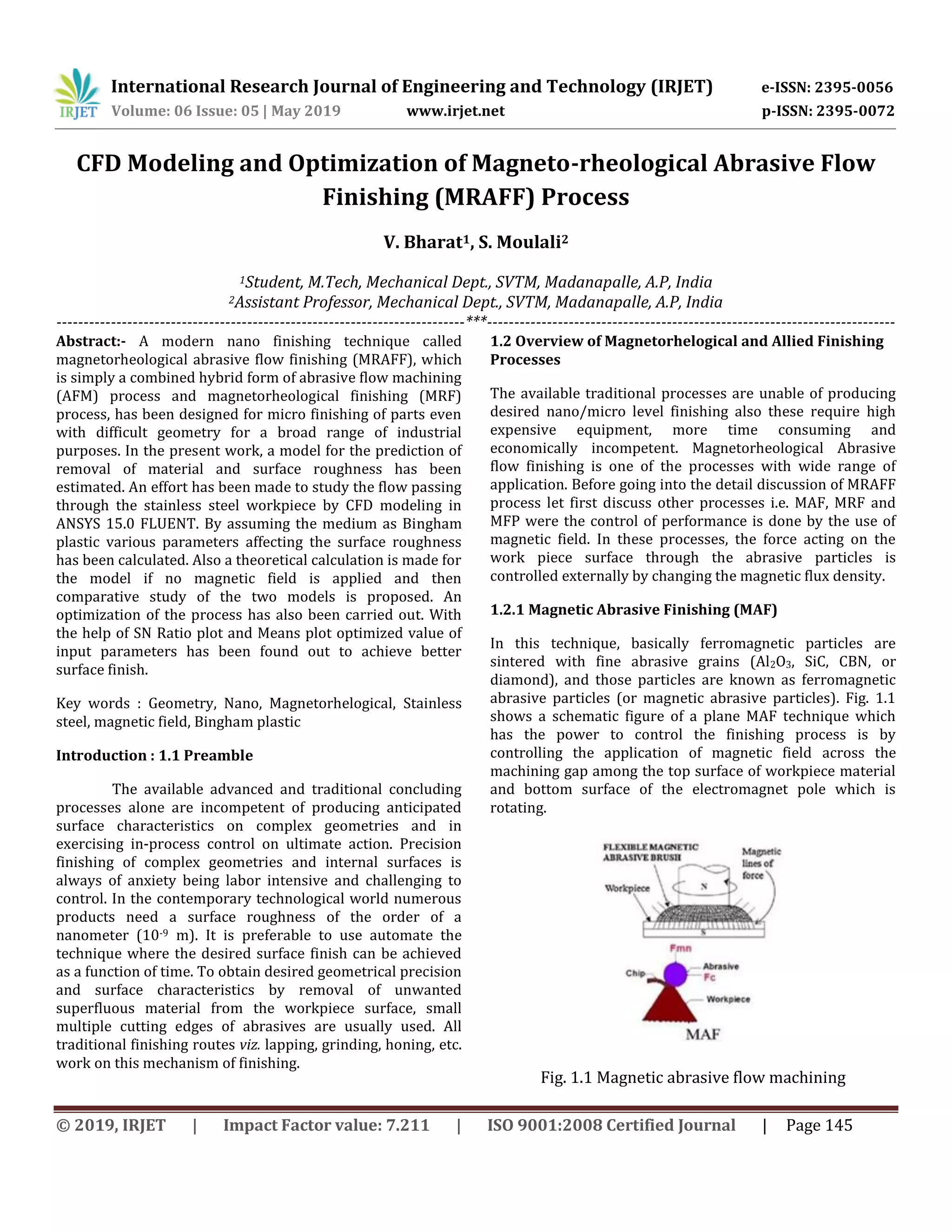
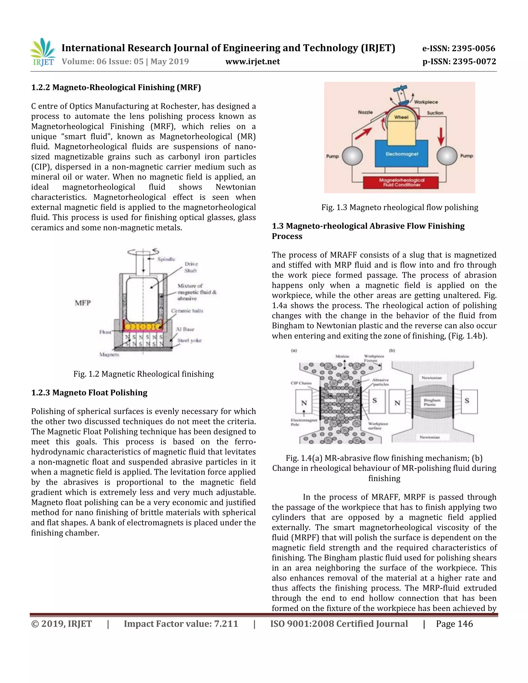

This document discusses modeling and optimizing the magneto-rheological abrasive flow finishing (MRAFF) process using computational fluid dynamics (CFD). It begins with an overview of the MRAFF process and similar processes like magnetic abrasive finishing and magneto-rheological finishing. It then describes modeling the MRAFF process using ANSYS 15.0 FLUENT to simulate the flow through a stainless steel workpiece and calculate parameters like surface roughness. An optimization of the process is carried out to determine input parameters that achieve the best surface finish. The document provides background on CFD modeling and its advantages over experimental testing before detailing the specific 2D CFD simulation conducted in this study of the MRAFF