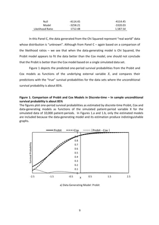
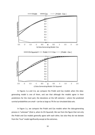
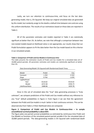
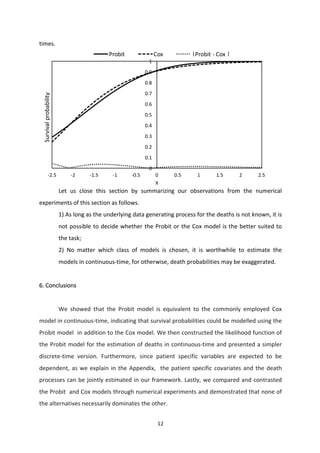
1	


The	
  Probit	
  Model	
  as	
  a	
  Continuous-­‐time	
  Survival	
  Model	


Eddie	
  Cruz,	
  Dylan	
  Lojac,	
  Deniz	
  Öncü,	
  	
  Becky	
  Turlip	


Math-­‐UA	
  251	
  
Introduction	
  to	
  Mathematical	
  Modelling	
  
May	
  9,	
  2016	


Abstract.	
  That	
  the	
  Probit	
  model	
  can	
  be	
  used	
  as	
  a	
  survival	
  model	
  in	
  discrete	
  time	
  is	
  well	
  
known.	
  We	
  show	
  that	
  the	
  Probit	
  model	
  can	
  be	
  used	
  as	
  a	
  survival	
  model	
  also	
  in	
  continuous	
  
time.	
   We	
   then	
   compare	
   and	
   contrast	
   the	
   predictions	
   of	
   the	
   Probit-­‐based	
   survival	
   model	
  
with	
  the	
  predictions	
  of	
  a	
  version	
  of	
  the	
  commonly	
  employed	
  Cox-­‐based	
  survival	
  model	
  on	
  a	
  
simple	
  set	
  of	
  simulated	
  data	
  in	
  discrete	
  as	
  well	
  as	
  in	
  continuous	
  time.	


1.	
  Introduction	
  
Although	
  it	
  appears	
  that	
  the	
  term	
  “survival	
  analysis”	
  originated	
  from	
  statistical	
  studies	
  in	
  
medicine	
   where	
   the	
   event	
   of	
   interest	
   was	
   “death”,	
   the	
   survival	
   analysis	
   can	
   be	
   used	
   for	
  
studying	
  any	
  process	
  for	
  which	
  the	
  outcome	
  variable	
  of	
  interest	
  is	
  the	
  time	
  until	
  an	
  event	
  
occurs.	
   Other	
   examples	
   include	
   the	
   arrival	
   time	
   of	
   equipment	
   failures,	
   traffic	
   accidents,	
  
stock	
  market	
  crashes,	
  default	
  of	
  borrowers,	
  unemployment	
  of	
  individuals	
  and	
  other	
  such	
  
events.	


   A	
   survival	
   model	
   can	
   be	
   characterized	
   by	
   a	
   stochastic	
   process	
   𝑍 𝑡 	
  which	
   takes	
  
values	
  from	
  a	
  set	
  of	
  two	
  states,	
  say,	
   1,2 	
  over	
  a	
  period	
   𝒯 = 0, 𝑇 	
  or	
   𝒯 = 0, 𝑇 	
  with	
   𝑇 ≤ ∞.	
  
We	
  assume	
  that	
  the	
  transition	
  probabilities	
  depend	
  on	
  a	
  time	
  varying	
  covariate	
  vector	
   𝑋 𝑡 	
  
and	
  that	
  the	
  first	
  entry	
  of	
  𝑋 𝑡 	
  	
  is	
  1.	
  We	
  assume	
  further	
  that	
  the	
  process	
  is	
  Markov	
  so	
  that	
  
the	
  transition	
  probabilities	
  from	
  state	
  𝑖	
  at	
  time	
  𝑠	
  to	
  state	
  𝑗	
  at	
  time	
  𝑡	
  where	
  𝑠 < 𝑡	
  depend	
  
only	
  on	
   𝑍 𝑠 	
  and	
   𝑋 𝑠 ,	
  and	
  are	
  independent	
  from	
  their	
  history	
  prior	
  to	
  time	
   𝑠.	
  That	
  is,	
  
𝑃45 𝑠, 𝑡 = 𝑃𝑟𝑜𝑏 𝑍 𝑡 = 𝑗 𝑍 𝑠 = 𝑖, 𝑋(𝑠) 	


  (1)	
  
2	


Since	
   we	
   are	
   interested	
   in	
   survival	
   models,	
   we	
   assume	
   that	
   the	
   state	
   1	
   is	
   the	
  
“survival”	
  state	
  and	
  the	
  state	
  2	
  is	
  the	
  “death”	
  state	
  so	
  that	
  𝑃;< 𝑠, 𝑡 = 0	
  and	
  𝑃;; 𝑠, 𝑡 = 1.	
  
The	
  survival	
  probability	
  from	
  time	
  𝑠	
  to	
  time	
  𝑡	
  is	
  then	
  𝑃<< 𝑠, 𝑡 = 𝑆(𝑠, 𝑡)	
  so	
  that	
  𝑃<; 𝑠, 𝑡 =
1 − 𝑆(𝑠, 𝑡).	
  The	
  function	
   𝑆 𝑡 = 𝑆(0, 𝑡)	
  is	
  called	
  the	
  survival	
  function.	


The	
  above	
  can	
  be	
  summarized	
  into	
  the	
  transition	
  probabilities	
  matrix	
   𝑷 𝑠, 𝑡 	
  as	
  
𝑷 𝑠, 𝑡 =
𝑃<<(𝑠, 𝑡) 𝑃<;(𝑠, 𝑡)
0 1
=
𝑆(𝑠, 𝑡) 1 − 𝑆(𝑠, 𝑡)
0 1


  (2)	
  
and,	
  since	
  the	
  process	
  is	
  Markov,	
  we	
  have	
  
𝑷 𝑠, 𝑢 = 	
  	
   𝑷 𝑠, 𝑡 𝑷 𝑡, 𝑢 ,	


   𝑠 < 𝑡 < 𝑢 ∈ 	
   𝒯.	


  (3)	
  
To	
  complete	
  the	
  model,	
  it	
  remains	
  to	
  specify	
  the	
  survival	
  probabilities	
   𝑆 𝑠, 𝑡 	
  or	
  the	
  survival	
  
function	
   𝑆 𝑡 	
  in	
  some	
  fashion.	
  We	
  do	
  this	
  after	
  the	
  next	
  section.	


2.	
  The	
  hazard	
  function	
  
An	
   alternative	
   characterization	
   of	
   the	
   model	
   is	
   given	
   by	
   the	
   hazard	
   function,	
   or	
  
instantaneous	
  rate	
  of	
  occurrence	
  of	
  the	
  event,	
  defined	
  in	
  our	
  formalization	
  as	
  
𝜆 𝑡 = lim∆G→I
𝑃<; 𝑡, 𝑡 + ∆𝑡
∆𝑡
.	


  (4)	


It	
  then	
  follows	
  from	
  the	
  ongoing	
  definitions,	
  and	
  the	
  equations	
  (2)	
  and	
  (3)	
  that	
  
𝑃<< 0, 𝑡 𝑃<; 𝑡, 𝑡 + ∆𝑡 = 𝑃<; 0, 𝑡 + ∆𝑡 − 𝑃<; 0, 𝑡 ,	


  (5)	
  
so	
  that	
  
𝑃<; 𝑡, 𝑡 + ∆𝑡 = −
𝑆 𝑡 + ∆𝑡 − 𝑆 𝑡
𝑆 𝑡
.	


  (6)	
  
Combining	
  the	
  equations	
  (4)	
  and	
  (6),	
  we	
  get	
  
𝜆 𝑡 = −
𝑑
𝑑𝑡
ln 𝑆 𝑡 	


  (7)	


3	


   We	
   are	
   almost	
   ready	
   to	
   discuss	
   some	
   alternative	
   specifications	
   of	
   the	
   survival	
  
function.	
  As	
  a	
  first	
  step	
  in	
  this	
  direction,	
  let	
  us	
  solve	
  the	
  equation	
  (7)	
  with	
  the	
  natural	
  initial	
  
condition1
	
   𝑆 0 = 1	
  to	
  get	
  
𝑆 𝑡 = exp − 𝜆 𝑠 𝑑𝑠
G
I
.	


  (8)	
  
It	
  should	
  be	
  mentioned	
  that	
  under	
  our	
  assumptions	
   𝜆 𝑠 	
  may	
  depend	
  on	
   𝑋 𝑠 	
  but	
  we	
  have	
  
been	
  supressing	
  this	
  dependence	
  for	
  convenience	
  all	
  along.	


   We	
  close	
  this	
  section	
  by	
  noting	
  that	
  an	
  alternative	
  way	
  of	
  characterizing	
  the	
  survival	
  
models	
  is	
  to	
  look	
  at	
  the	
  probability	
  distribution	
  function	
  of	
  a	
  continuous	
  random	
  variable	
  
𝜏 ∈ 𝒯	
  with	
  the	
  probability	
  density	
  function	
   𝑓(𝑡)	
  and	
  the	
  cumulative	
  distribution	
  function	
  
𝐹(𝑡)	
   which	
   gives	
   the	
   probability	
   that	
   the	
   event	
   has	
   occurred	
   by	
   time	
   𝑡 > 𝜏,	
  	
   𝑡 ∈ 𝒯.	
   It	
   is	
  
evident	
  that	
   𝑆 𝑡 = 1 − 𝐹(𝑡)	
  and	
  it	
  follows	
  from	
  the	
  equation	
  (7)	
  that	
  
𝑓 𝑡 = 𝜆 𝑡 𝑆 𝑡 .	


  (9)	


3.	
  Two	
  alternatives	
  
In	
  view	
  of	
  Sections	
  1	
  and	
  2,	
  we	
  have	
  two	
  alternatives.	
  We	
  can	
  specify	
  either	
  the	
  hazard	
  
function	
   𝜆 𝑡 	
   or	
   the	
   survival	
   function	
   𝑆(𝑡).	
   The	
   Cox	
   model	
   is	
   one	
   of	
   the	
   commonly	
  
employed	
   approaches	
   for	
   specifying	
   the	
   hazard	
   function.	
   Since	
   we	
   are	
   interested	
   in	
   the	
  
influence	
  of	
  a	
  time	
  varying	
  covariate	
  vector	
   𝑋 𝑡 	
  on	
  the	
  survival	
  probabilities,	
  we	
  adopt	
  the	
  
following	
  version	
  of	
  the	
  Cox	
  model:	
  
	
   𝜆 𝑡 = exp 	
  { 𝛼′𝑋(𝑡)},	


  (10)	
  
where	
   𝛼	
  is	
  a	
  vector	
  of	
  parameters.	


   The	
  second	
  alternative	
  is	
  specifying	
  the	
  survival	
  function	
  directly.	
  Let	
  Φ ∙ 	
  be	
  the	
  
cumulative	
   distribution	
   function	
   of	
   some	
   distribution	
   whose	
   probability	
   distribution	
  
function	
   is	
   𝜙 ∙ .	
   Although	
   any	
   distribution	
   might	
   do,	
   we	
   assume	
   that	
   the	
   Φ ∙ 	
   is	
   the	
  
cumulative	
  distribution	
  function	
  of	
  the	
  standard	
  normal	
  distribution	
  and	
  specify	
  the	
  survival	
  
function	
  as	
  
𝑆 𝑡 = Φ 𝜇 𝑡 ,	


  (11)	
  
where	
   𝜇 𝑡 	
  is	
  a	
  cut-­‐off	
  function.	
  This	
  is	
  a	
  Probit	
  specification.	


1
	
  Otherwise,	
  there	
  is	
  nothing	
  to	
  observe.	
  
4	


Our	
  main	
  reason	
  for	
  choosing	
  Probit	
  is	
  that	
  it	
  provides	
  a	
  simple	
  tool	
  for	
  the	
  joint	
  
estimation	
   of	
   death	
   and	
   the	
   covariates,	
   as	
   we	
   describe	
   on	
   a	
   simple	
   example	
   in	
   the	
  
Appendix.	
  For	
  other	
  specifications,	
  the	
  joint	
  estimation	
  of	
  death	
  and	
  the	
  covariates	
  might	
  be	
  
very	
  difficult,	
  if	
  not	
  impossible.	
  Why	
  this	
  is	
  important	
  is	
  explained	
  in	
  the	
  Appendix	
  as	
  well.	


Note	
  that	
  given	
  the	
  properties	
  of	
  the	
  survival	
  function	
   𝑆(𝑡),	
  the	
  cut-­‐off	
  function	
   𝜇 𝑡 	
  
must	
  be	
  decreasing	
  and	
  we	
  must	
  have	
  lim
G→I
𝜇 𝑡 = ∞.	
  From	
  the	
  equations	
  (7)	
  and	
  (11),	
  we	
  
see	
  also	
  that	
  
𝜆 𝑡 = −
𝜙 𝜇 𝑡 𝜇′ 𝑡
Φ 𝜇(𝑡)


  (12)	
  
which	
   verifies	
   that	
   𝜇 𝑡 	
   must	
   be	
   decreasing.	
   We	
   defer	
   the	
   specification	
   of	
   the	
   cut-­‐off	
  
function	
  to	
  the	
  next	
  section.	
  In	
  closing	
  this	
  section,	
  we	
  note	
  that	
  the	
  survival	
  probability	
  
from	
  time	
   𝑠	
  to	
  time	
   𝑡	
  should	
  take	
  the	
  form	
  
𝑆 𝑠, 𝑡 = Φ 𝜇b(𝑡 − 𝑠) 	


  (13)	
  
where	
   𝜇b(∙)	
  is	
  the	
  cut-­‐off	
  function	
  associated	
  with	
  time	
  s.	
  Of	
  course,	
   𝜇b ∙ 	
  must	
  have	
  the	
  
same	
  properties	
   𝜇 ∙ 	
  has.	


4.	
  The	
  setup	
  
In	
  what	
  follows,	
  we	
  will	
  consider	
  a	
  set	
  of	
   𝑀	
  “entities”	
  such	
  as	
  patients	
  or	
  firms	
  or	
  machines	
  
and	
  the	
  like,	
  and	
  study	
  their	
  failure	
  probabilities.	
  In	
  the	
  case	
  of	
  patients,	
  the	
  failure	
  can	
  be	
  
death;	
  in	
  the	
  case	
  of	
  firms,	
  it	
  can	
  be	
  default	
  on	
  debt	
  and	
  so	
  on	
  so	
  forth.	
  For	
  simplicity	
  in	
  
discussion,	
  we	
  will	
  refer	
  to	
  all	
  of	
  these	
  as	
  patients	
  and	
  our	
  failure	
  of	
  interest	
  will	
  be	
  death.	
  
We	
  will	
  begin	
  with	
  a	
  single	
  patient	
  and	
  extend	
  our	
  results	
  to	
   𝑀	
  patients	
  later.	


4.1.	
  A	
  single	
  patient	
  
In	
  this	
  subsection,	
  we	
  will	
  look	
  at	
  a	
  single	
  patient	
  and	
  assume	
  that	
  the	
  covariates	
  𝑋(𝑡)	
  are	
  
sampled	
  with	
  intervals	
  of	
  equal	
  length	
  ∆𝑡.2
	
  Suppose	
  now	
  that	
  the	
  observations	
  were	
  made	


2
	
   Note	
   that	
   although	
   the	
   assumption	
   that	
   the	
   covariates	
   sampled	
   with	
   intervals	
   of	
   equal	
   length	
   is	
   not	
  
necessary,	
  it	
  will	
  simplify	
  the	
  formulation.	
  Our	
  results	
  can	
  easily	
  be	
  extended	
  to	
  the	
  case	
  of	
  unequal	
  length	
  
sampling	
  intervals	
  after	
  minor	
  modifications.	
  
5	


in	
   the	
   interval	
   [0, 𝑇]	
   where	
   𝑇 = 𝑁∆𝑡	
  and	
   𝑁	
   is	
   the	
   number	
   of	
   intervals.	
   Let	
   us	
   set	
   𝑡4 =
𝑖∆𝑡, 𝑖 = 0,1, … , 𝑁.	
   	
   Since	
   the	
   sampling	
   is	
   done	
   discretely,	
   further	
   suppose	
   that	
   𝑋 𝑡 =
𝑋(𝑡4i<)	
   =𝑋Gjkl
for	
   any	
   𝑡 ∈ [𝑡4i<, 𝑡4),	
   𝑖 = 1, … , 𝑁.	
   With	
   this	
   assumption,	
   we	
   have	
   also	
   that	
  
𝜆 𝑡 = 𝜆 𝑡4i< =	
   𝜆Gjkl
	
  for	
  any	
   𝑡 ∈ [𝑡4i<, 𝑡4),	
   𝑖 = 1, … , 𝑁.	


Let	
  us	
  now	
  assume	
  that	
  either	
  at	
  some	
  time	
   𝜏 ∈ [𝑡mi<, 𝑡m)	
  for	
  some	
   𝑘,	
  0 < 𝑘 ≤ 𝑁,	
  
that	
  is,	
  in	
  the	
  𝑘Go
period,	
  the	
  death	
  occurred	
  or	
  that	
  the	
  patient	
  survived	
  in	
  the	
  observation	
  
interval	
   0, 𝑇 .	
   If	
   the	
   survival	
   occurred	
   in	
   0, 𝑇 ,	
   set	
   𝜏 = 𝑡m	
   and	
   𝑘 = 𝑁.	
   Lastly,	
   define	
   the	
  
indicator	
  variables	
   𝑌5 𝑡 = 1 𝑍 𝑡 = 𝑗 , 𝑗 = 1,2.	
  	
  This	
  means	
  that	
  if	
   𝑌<(𝑡) =1	
  at	
  time	
   𝑡 ∈
[0, 𝑇]	
  ,	
  the	
  patient	
  survived	
  until	
  time	
   𝑡.	
  Otherwise,	
   𝑌;(𝑡) =1	
  and	
  the	
  patient	
  is	
  dead	
  at	
  time	
  
𝑡.	


   Under	
  these	
  assumptions,	
  from	
  the	
  equation	
  (8)	
  we	
  have	
  
𝑆 𝜏 = 𝑆 𝑡mi<, 𝜏 𝑆 𝑡I, 𝑡mi< 	
  ,	


  (14)	
  
where	
  
𝑆 𝑡4i<, 𝑡4 = exp −	
   𝜆Gjkl
	
  Δ 𝑡 , 𝑖 = 1,2, … , 𝑘 − 1,	


  (15)	
  
𝑆 𝑡mi<, 𝜏 = exp −𝜆Grkl
(τ − 𝑡mi<) ,	


  (16)	
  
and	
  	
  
𝑆 𝑡I, 𝑡mi< 	
  = 𝑆 𝑡4i<, 𝑡4
mi<
4t<
,	


  (17)	


Given	
  these,	
  we	
  have	
  two	
  alternatives.	


4.1.1.	
  The	
  discrete	
  case	
  
The	
   first	
   alternative	
   is	
   to	
   ignore	
   that	
   the	
   death	
   occurred	
   in	
   the	
   interior	
   of	
   the	
   interval	
  
[𝑡mi<, 𝑡m),	
  set	
   𝜏 = 𝑡m.	
  Then	
  the	
  associated	
  likelihood	
  function	
  for	
  this	
  patient	
  is	
  	
  
ℒv 𝜃 = 𝑌< 𝑡m 𝑆 𝑡mi<, 𝑡m + 𝑌; 𝑡m [1 − 𝑆 𝑡mi<, 𝑡m ] 𝑆 𝑡I, 𝑡mi< ,	


  (17)	
  
where	
   𝜃	
  is	
  the	
  parameter	
  vector	
  to	
  be	
  estimated	
  once	
  the	
  modelling	
  approach	
  is	
  chosen.	


6	


If	
  we	
  choose	
  to	
  model	
  the	
  𝜆Gj
	
  as	
  in	
  the	
  version	
  of	
  Cox	
  model	
  given	
  by	
  the	
  equation	
  
(10),	
  then	
   𝜃 = 𝛼	
  and	
  we	
  are	
  done.	
  If,	
  instead,	
  we	
  choose	
  to	
  model	
  the	
  survival	
  probabilities	
  
𝑆 𝑡4i<, 𝑡4 , 𝑖 = 1,2, … , 𝑘,	
  then	
  we	
  can	
  proceed	
  as	
  follows.	


Set	
   𝜇Gjkl
= 𝜇Gjkl
𝑡4 − 𝑡4i< , 𝑖 = 1,2, … , 𝑘	
  and	
  model	
  the	
   𝜇Gjkl
as	
  
𝜇Gjkl
= 𝛽y
𝑋Gjkl
.	


  (18)	
  
In	
  this	
  case,	
  the	
  parameter	
  vector	
   𝜃 = 𝛽	
  and	
  the	
  survival	
  probabilities	
  are	
  
𝑆 𝑡4i<, 𝑡4 = Φ 𝜇Gjkl
.	


  (19)	
  
We	
  can	
  now	
  rewrite	
  the	
  likelihood	
  function	
  for	
  this	
  patient	
  as	
  
ℒv 𝜃 = 𝑌< 𝑡m Φ 𝜇Grkl
+ 𝑌; 𝑡m [1 − Φ 𝜇Grkl
] Φ 𝜇Gjkl
mi<
4t<
,	


  (20)	
  
which	
  is	
  the	
  usual	
  likelihood	
  function	
  of	
  the	
  Probit	
  model	
  in	
  discrete	
  time.	


4.1.2.	
  The	
  continuous	
  case	
  
If	
  we	
  do	
  not	
  ignore	
  that	
  the	
  death	
  occurred	
  in	
  the	
  interior	
  of	
  the	
  interval	
  [𝑡mi<, 𝑡m)	
  and	
  
recall	
  from	
  the	
  equation	
  (9)	
  that	
   𝑓 𝜏 = 𝜆 𝜏 𝑆(𝜏),	
  then	
  from	
  the	
  ongoing	
  development	
  the	
  
likelihood	
  function	
  for	
  this	
  patient	
  is	
  
ℒz 𝜃 = {𝑌< 𝜏 + 𝑌; 𝜏 𝜆Grkl
}𝑆 𝑡mi<, 𝜏 𝑆 𝑡I, 𝑡mi< .	


  (21)	
  
If	
  we	
  choose	
  to	
  model	
  the	
  hazard	
  function	
  as	
  in	
  the	
  above	
  Cox-­‐based	
  formulation,	
  we	
  are	
  
done	
   already.	
   The	
   equations	
   (10),	
   (15)	
   and	
   (16)	
   complete	
   the	
   model	
   and	
   the	
   parameter	
  
vector	
  to	
  be	
  estimated	
  is	
   𝜃 = 𝛼.	


   Let	
   us	
   now	
   proceed	
   to	
   the	
   Probit	
   formulation	
   and	
   observe	
   from	
   the	
   ongoing	
  
development	
  that	
  
exp −	
   𝜆Grkl
	
  Δ 𝑡 = 𝑆 𝑡mi<, 𝑡m = Φ 𝜇Grkl
.	


  (22)	
  
Then,	
  
𝜆Grkl
=
1
Δ𝑡
ln
1
Φ 𝜇Grkl
,	


  (23)	
  
and	
  
𝑆 𝑡mi<, 𝜏 = Φ 𝜇Grkl
{iGrkl
|G .	


  (24)	
  
7	


Combining	
   all	
   of	
   the	
   above	
   gives	
   us	
   the	
   Probit	
   version	
   of	
   the	
   continuous	
   time	
   likelihood	
  
function	
  for	
  this	
  patient.	
  It	
  is	
  
ℒz 𝜃 = 𝑌< 𝜏 + 𝑌; 𝜏 ln
1
Φ 𝜇Grkl
Φ 𝜇Grkl
{iGrkl
|G Φ 𝜇Gjkl
mi<
4t<
.	


  (25)	
  
Now,	
  the	
  parameter	
  vector	
  to	
  be	
  estimated	
  is	
   𝜃 = 𝛽.	


4.2.	
  Many	
  patients	


Extension	
  to	
  the	
  case	
  of	
  multiple	
  patients	
  is	
  trivial.	
  Index	
  all	
  of	
  the	
  relevant	
  variables	
  with	
  
𝑚 = 1,2, …	
  , 𝑀	
  and	
  denote	
  by	
  ℒ~ 𝜃 	
  a	
  generic	
  for	
  all	
  of	
  the	
  likelihood	
  functions	
  written	
  
above	
  for	
  the	
   𝑚Go
	
  patient.	
  Then	
  the	
  likelihood	
  function	
  ℒ 𝜃 	
  associated	
  with	
  our	
  patient	
  
sample	
  is	
  	
  
ℒ 𝜃 = ℒ~ 𝜃
•
~t<
.	


  (26)	
  
And	
  we	
  are	
  done.	


5.	
  	
  Numerical	
  Experiments	


   In	
   this	
   section,	
   we	
   compare	
   and	
   contrast	
   the	
   predictions	
   of	
   the	
   Probit	
   and	
   Cox	
  	
  
models	
  for	
  four	
  simulated	
  data	
  sets	
  of	
  10,000	
  firm-­‐periods.	
  We	
  set	
  the	
  data	
  sampling	
  period	
  
length	
   as	
   ∆𝑡=1	
   for	
   convenience,	
   suppose	
   there	
   is	
   an	
   external	
   variable	
   𝑋	
  that	
   drives	
   the	
  
defaults,	
   and	
   draw	
   10,000	
   values	
   for	
   𝑋	
   assuming	
   that	
   it	
   is	
   identically	
   and	
   independently	
  
distributed	
  standard	
  normal.	
  	
  
Finally,	
  we	
  generate	
  our	
  data	
  from	
  the	
  following	
  three	
  models	
  that	
  give	
  the	
  survival	
  
probabilities	
  as	
  follows.	
  
a)	
  Probit:	


   𝑃<<(0,1) = Φ 1.45 + 𝑋 ,	


b)	
  Cox:	


   𝑃<<(0,1) = exp −exp	
  (2.17 − 𝑋) ,	


c)	
  Chi	
  Squared:	
   	
  	
   𝑃<<(0,1) = Χ;
exp(1 + 𝑋) ,	


In	
  the	
  above,	
  Φ ∙ 	
  and	
  	
  Χ;
∙ 	
  and	
  are	
  the	
  cumulative	
  distribution	
  functions	
  of	
  the	
  standard	
  
normal	
  and	
  Chi	
  Squared	
  with	
  unit	
  degree	
  of	
  freedom	
  distributions.	
  We	
  chose	
  the	
  parameter	
  
8	


values	
   of	
   the	
   models	
   in	
   such	
   a	
   way	
   that	
   the	
   resulting	
   in-­‐sample	
   unconditional	
   survival	
  
probabilities	
  in	
  the	
  data	
  sets	
  are	
  about	
  85%.	
  
	
   Next,	
  we	
  estimate	
  the	
  models	
  for	
  each	
  of	
  the	
  data	
  sets	
  under	
  the	
  assumption	
  that	
  
the	
  observations	
  are	
  made	
  in	
  discrete-­‐time.	
  Table	
  1	
  summarizes	
  the	
  estimation	
  results.	
  All	
  
parameter	
  estimates	
  and	
  models	
  are	
  statistically	
  significant	
  at	
  better	
  than	
  1%.	
  Although	
  a	
  
comparison	
  of	
  models	
  based	
  on	
  the	
  likelihood	
  ratios	
  is	
  not	
  a	
  proper	
  comparison	
  for	
  non-­‐
nested	
   models,	
   we	
   nevertheless	
   see	
   from	
   this	
   comparison	
   in	
   Panels	
   A	
   and	
   B	
   that	
   when	
  
Probit	
  is	
  the	
  data-­‐generating	
  model,	
  Probit	
  appears	
  to	
  fit	
  the	
  data	
  better	
  than	
  Cox,	
  whereas	
  
when	
   Cox	
   is	
   the	
   data-­‐generating	
   model,	
   Cox	
   appears	
   to	
   fit	
   the	
   data	
   better	
   than	
   Probit.	
  
These	
  results	
  are	
  expected	
  and	
  included	
  only	
  as	
  a	
  check	
  on	
  our	
  results.	


Table	
  1.	
  Comparison	
  of	
  Probit	
  and	
  Cox	
  Models	
  in	
  Discrete-­‐time	
  
This	
  table	
  presents	
  the	
  estimation	
  results	
  of	
  Probit	
  and	
  Cox	
  models	
  for	
  three	
  simulated	
  data	
  sets	
  of	
  
10,000	
   patient-­‐periods.	
   All	
   parameter	
   estimates	
   and	
   models	
   are	
   statistically	
   significant	
   at	
   better	
  
than	
  1%.	


Panel	
  A.	
  Data	
  Generating	
  Model:	
  Probit	


  Model	
   Probit	
   Cox	
  
Constant	
   1.473	
   -­‐2.554	
  
Slope	
  	
   0.993	
   -­‐1.427	
  
Loglikelihood	


  Null	
   -­‐4185.23	
   -­‐4185.23	


  Model	
   -­‐2975.39	
   -­‐3009.39	
  
Likelihood	
  Ratio	
   2419.68	
   2351.68	


Panel	
  B.	
  Data	
  Generating	
  Model:	
  Cox	


  Model	
   Probit	
   Cox	
  
Constant	
   1.232	
   -­‐2.214	
  
Slope	
  	
   0.608	
   -­‐0.980	
  
Loglikelihood	


  Null	
   -­‐4155.31	
   -­‐4155.31	


  Model	
   -­‐3548.29	
   -­‐3541.40	
  
Likelihood	
  Ratio	
   1,214.06	
   1,227.82	


Panel	
  C.	
  Data	
  Generating	
  Model:	
  Chi	
  Squared	


  Model	
   Probit	
   Cox	
  
Constant	
   1.355	
   -­‐2.339	
  
Slope	
  	
   0.783	
   -­‐1.101	
  
Loglikelihood	


9	


  Null	
   -­‐4114.45	
   -­‐4114.45	


  Model	
   -­‐3258.21	
   -­‐3320.03	
  
Likelihood	
  Ratio	
   1712.48	
   1,587.54	


In	
  this	
  Panel	
  C,	
  the	
  data	
  generated	
  from	
  the	
  Chi	
  Squared	
  represent	
  “real	
  world”	
  data	
  
whose	
  distribution	
  is	
  “unknown”.	
  Although	
  from	
  Panel	
  C	
  –	
  again	
  based	
  on	
  a	
  comparison	
  of	
  
the	
   likelihood	
   ratios	
   –	
   we	
   see	
   that	
   when	
   the	
   data-­‐generating	
   model	
   is	
   Chi	
   Squared,	
   the	
  
Probit	
  model	
  appears	
  to	
  fit	
  the	
  data	
  better	
  than	
  the	
  Cox	
  model,	
  one	
  should	
  not	
  conclude	
  
that	
  the	
  Probit	
  is	
  better	
  than	
  the	
  Cox	
  model	
  based	
  on	
  a	
  single	
  simulated	
  data	
  set.	
  
Figure	
  1	
  depicts	
  the	
  predicted	
  one-­‐period	
  survival	
  probabilities	
  from	
  the	
  Probit	
  and	
  
Cox	
   models	
   as	
   functions	
   of	
   the	
   underlying	
   external	
   variable	
   𝑋,	
   and	
   compares	
   their	
  
predictions	
  with	
  the	
  “true”	
  survival	
  probabilities	
  for	
  the	
  data	
  sets	
  where	
  the	
  unconditional	
  
survival	
  probability	
  is	
  about	
  85%.	


Figure	
  1.	
  Comparison	
  of	
  Probit	
  and	
  Cox	
  Models	
  in	
  Discrete-­‐time	
  –	
  In	
  sample	
  unconditional	
  
survival	
  probability	
  is	
  about	
  85%	
  
The	
  figures	
  plot	
  one-­‐period	
  survival	
  probabilities	
  as	
  estimated	
  by	
  discrete-­‐time	
  Probit,	
  Cox	
  and	
  
data-­‐generating	
   models	
   as	
   functions	
   of	
   the	
   simulated	
   patient-­‐period	
   variable	
   X	
   for	
   the	
  
simulated	
  data	
  of	
  10,000	
  patient-­‐periods.	
  	
  In	
  Figures	
  1.a	
  and	
  1.b,	
  only	
  the	
  estimated	
  models	
  
are	
  included	
  because	
  the	
  data-­‐generating	
  model	
  and	
  its	
  estimation	
  produce	
  indistinguishable	
  
graphs.	


a)	
  Data	
  Generating	
  Model:	
  Probit	


0
0.1
0.2
0.3
0.4
0.5
0.6
0.7
0.8
0.9
1
-­‐2.5 -­‐1.5 -­‐0.5 0.5 1.5 2.5
Survival	
  Probability
X
Probit Cox │Probit	
  -­‐ Cox	
  │
10	


b)	
  Data	
  Generating	
  Model:	
  Cox	


c)	
  Data	
  Generating	
  Model:	
  Chi	
  Squared	


   In	
   Figures	
   1.a	
   and	
   1.b,	
   we	
   compare	
   the	
   Probit	
   and	
   Cox	
   models	
   when	
   the	
   data-­‐
generating	
   model	
   is	
   one	
   of	
   them,	
   and	
   see	
   that	
   although	
   the	
   models	
   agree	
   in	
   their	
  
predictions	
   for	
   the	
   most	
   part,	
   the	
   deviations	
   at	
   the	
   left	
   extreme	
   –	
   where	
   the	
   predicted	
  
survival	
  probabilities	
  are	
  small	
  –	
  can	
  be	
  as	
  large	
  as	
  7%	
  for	
  our	
  simulated	
  data	
  sets.	


   In	
   Figure	
   1.c,	
   we	
   compare	
   the	
   Probit	
   and	
   Cox	
   models	
   when	
   the	
   data-­‐generating	
  
process	
  is	
  “unknown”	
  (that	
  is,	
  when	
  its	
  Chi	
  Squared).	
  We	
  see	
  from	
  the	
  figure	
  that	
  not	
  only	
  
the	
  Probit	
  and	
  Cox	
  models	
  generally	
  agree	
  with	
  each	
  other,	
  but	
  also	
  they	
  do	
  not	
  deviate	
  
from	
  the	
  “true”	
  model	
  significantly	
  except	
  at	
  the	
  extremes.	
  	
  
0
0.1
0.2
0.3
0.4
0.5
0.6
0.7
0.8
0.9
1
-­‐2.5 -­‐2 -­‐1.5 -­‐1 -­‐0.5 0 0.5 1 1.5 2 2.5
Survival	
  probability
X
Probit Cox │Probit	
  -­‐ Cox	
  │
0
0.1
0.2
0.3
0.4
0.5
0.6
0.7
0.8
0.9
1
-­‐2.5 -­‐2 -­‐1.5 -­‐1 -­‐0.5 0 0.5 1 1.5 2 2.5
Survival	
  Probability
X
Chi	
  Squared Probit Cox │Probit	
  -­‐ Cox	
  │
11	


   Lastly,	
   we	
   turn	
   our	
   attention	
   to	
   continuous-­‐time,	
   and	
   focus	
   on	
   the	
   last	
   data-­‐
generating	
  model,	
  that	
  is,	
  Chi	
  Squared.	
  We	
  keep	
  our	
  original	
  simulated	
  data	
  set	
  generated	
  
by	
  this	
  model,	
  but	
  randomly	
  assign	
  to	
  the	
  deaths	
  a	
  default	
  time	
  between	
  zero	
  and	
  one	
  using	
  
the	
  uniform	
  distribution.	
  The	
  results	
  of	
  our	
  estimations	
  based	
  on	
  these	
  data	
  are	
  reported	
  in	
  
Table	
  2.	


All	
   of	
   the	
   parameter	
   estimates	
   and	
   models	
   reported	
   in	
   Table	
   2	
   are	
   statistically	
  
significant	
  at	
  better	
  than	
  1%.	
  As	
  before,	
  we	
  note	
  that	
  although	
  a	
  comparison	
  between	
  two	
  
non-­‐nested	
  models	
  based	
  on	
  likelihood	
  ratios	
  is	
  not	
  appropriate,	
  our	
  results	
  show	
  that	
  our	
  
Probit	
  formulation	
  appears	
  to	
  fit	
  the	
  data	
  better	
  than	
  the	
  Cox	
  model	
  based	
  on	
  this	
  criterion	
  
in	
  our	
  simulated	
  sample.	


Table	
  2.	
  Comparison	
  of	
  Probit	
  and	
  Cox	
  Models	
  in	
  Continuous-­‐time	
  
This	
   table	
   presents	
   the	
   estimation	
   results	
   of	
   Probit	
   and	
   Cox	
   models	
   for	
   a	
   simulated	
   data	
   set	
   of	
  
10,000	
   patient-­‐periods.	
   All	
   parameter	
   estimates	
   and	
   models	
   are	
   statistically	
   significant	
   at	
   better	
  
than	
  1%.	


Data	
  Generating	
  Model:	
  Chi	
  Squared	
  with	
  Randomized	
  Death	
  Times	


  Model	
   Probit	
   Cox	
  
Constant	
   1.354	
   -­‐2.333	
  
Slope	
  	
   0.764	
   -­‐1.070	
  
Loglikelihood	


  Null	
   -­‐4116.62	
   -­‐4116.62	


  Model	
   -­‐3272.58	
   -­‐3336.73	
  
Likelihood	
  Ratio	
   1688.08	
   1659.78	


Since	
   in	
   this	
   set	
   of	
   simulated	
   data	
   the	
   “true”	
   data	
   generating	
   processes	
   is	
   “truly	
  
unknown”,	
  we	
  compare	
  predictions	
  of	
  the	
  Probit	
  and	
  Cox	
  models	
  without	
  any	
  reference	
  to	
  
any	
   “true”	
   default	
   probabilities	
   in	
   Figure	
   2.	
   From	
   Figure	
   2	
   we	
   see	
   that	
   the	
   agreement	
  
between	
  the	
  Probit	
  and	
  Cox	
  models	
  is	
  much	
  	
  better	
  in	
  their	
  continuous	
  versions.	
  This	
  can	
  be	
  
observed	
  also	
  from	
  Table	
  2,	
  if	
  their	
  likelihood	
  ratios	
  are	
  compared.	
  
Figure	
   2.	
   Comparison	
   of	
   Probit	
   and	
   Cox	
   Models	
   in	
   Continuous-­‐time	
   –	
   In	
   sample	
  
unconditional	
  survival	
  probability	
  is	
  about	
  85%	
  
The	
  figure	
  plots	
  one-­‐period	
  survival	
  probabilities	
  as	
  estimated	
  by	
  continuous-­‐time	
  Probit	
  and	
  
Cox	
  Models	
  as	
  functions	
  of	
  the	
  simulated	
  pazient-­‐period	
  variable	
  X	
  for	
  the	
  simulated	
  data	
  of	
  
10,000	
  patient-­‐periods.	
  	
  The	
  data-­‐generating	
  models	
  is	
  Chi	
  Squared	
  with	
  randomized	
  death	
  
12	


times.	


Let	
   us	
   close	
   this	
   section	
   by	
   summarizing	
   our	
   observations	
   from	
   the	
   numerical	
  
experiments	
  of	
  this	
  section	
  as	
  follows.	
  
1)	
  As	
  long	
  as	
  the	
  underlying	
  data	
  generating	
  process	
  for	
  the	
  deaths	
  is	
  not	
  known,	
  it	
  is	
  
not	
  possible	
  to	
  decide	
  whether	
  the	
  Probit	
  or	
  the	
  Cox	
  model	
  is	
  the	
  better	
  suited	
  to	
  
the	
  task;	
  
2)	
   No	
   matter	
   which	
   class	
   of	
   models	
   is	
   chosen,	
   it	
   is	
   worthwhile	
   to	
   estimate	
   the	
  
models	
  in	
  continuous-­‐time,	
  for	
  otherwise,	
  death	
  probabilities	
  may	
  be	
  exaggerated.	


6.	
  Conclusions	


We	
   showed	
   that	
   the	
   Probit	
   model	
   is	
   equivalent	
   to	
   the	
   commonly	
   employed	
   Cox	
  
model	
  in	
  continuous-­‐time,	
  indicating	
  that	
  survival	
  probabilities	
  could	
  be	
  modelled	
  using	
  the	
  
Probit	
  model	
  	
  in	
  addition	
  to	
  the	
  Cox	
  model.	
  We	
  then	
  constructed	
  the	
  likelihood	
  function	
  of	
  
the	
  Probit	
  model	
  for	
  the	
  estimation	
  of	
  deaths	
  in	
  continuous-­‐time	
  and	
  presented	
  a	
  simpler	
  
discrete-­‐time	
   version.	
   Furthermore,	
   since	
   patient	
   specific	
   variables	
   are	
   expected	
   to	
   be	
  
dependent,	
  as	
  we	
  explain	
  in	
  the	
  Appendix,	
  	
  the	
  patient	
  specific	
  covariates	
  and	
  the	
  death	
  
processes	
  can	
  be	
  jointly	
  estimated	
  in	
  our	
  framework.	
  Lastly,	
  we	
  compared	
  and	
  contrasted	
  
the	
  Probit	
  	
  and	
  Cox	
  models	
  through	
  numerical	
  experiments	
  and	
  demonstrated	
  that	
  none	
  of	
  
the	
  alternatives	
  necessarily	
  dominates	
  the	
  other.	
  	
  
0
0.1
0.2
0.3
0.4
0.5
0.6
0.7
0.8
0.9
1
-­‐2.5 -­‐2 -­‐1.5 -­‐1 -­‐0.5 0 0.5 1 1.5 2 2.5
Survival	
  probability
X
Probit Cox │Probit	
  -­‐ Cox	
  │
13	


14	


Appendix	
  
As	
  we	
  mentioned	
  in	
  Section	
  3,	
  one	
  advantage	
  of	
  our	
  Probit	
  formulation	
  is	
  that	
  it	
  provides	
  a	
  
simple	
  tool	
  for	
  the	
  joint	
  estimation	
  of	
  death	
  and	
  the	
  covariates.	
  	
  To	
  explain	
  why	
  the	
  joint	
  
estimation	
  of	
  death	
  and	
  the	
  covariates	
  is	
  important,	
  consider	
  a	
  set	
  of	
  patients	
  and	
  suppose	
  
that	
  the	
  covariates	
  are	
  some	
  patient	
  related	
  variables	
  that	
  are	
  recorded	
  during	
  doctor	
  visits.	
  
For	
  convenience,	
  focus	
  on	
  a	
  single	
  patient	
  and	
  suppose	
  that	
  there	
  is	
  one	
  patient	
  specific	
  
variable,	
  say,	
   𝐵 𝑡 .	


Recall	
  that	
  state	
  1	
  is	
  the	
  survival	
  state	
  and	
  state	
  2	
  is	
  the	
  death	
  state,	
  and	
  focus	
  on	
  
two	
   observations	
   in	
   discrete-­‐time,	
   at	
   times	
   𝑡 = 𝑡I	
   and	
   𝑡 = 𝑡< > 𝑡I.	
   The	
   process	
   𝑍(𝑡)	
   is	
  
initialized	
  at	
   𝑡 = 𝑡I	
  as	
   𝑍 𝑡I = 1	
  and	
  the	
  latent	
  process	
   𝑍∗
(𝑡)	
  determines	
  the	
  next	
  state	
  
according	
  as	
  
𝑍 𝑡< = 1,	


   𝑖 𝑓	
  	
  	
   𝑍∗
𝑡< ≤ 𝑎	


  and	


   𝑍 𝑡< = 2,	


   𝑖 𝑓	
  	
  	
   𝑍∗
𝑡< > 𝑎	


  ( 𝐴. 1)	
  
For	
  further	
  simplicity,	
  consider	
  the	
  following	
  processes:	
  
	
   𝐵 𝑡< = 𝑏 + 𝜂	


  ( 𝐴. 2)	
  
𝑍∗
𝑡< = 𝜖	


  ( 𝐴. 3)	
  
where	
  𝑏	
  is	
  some	
  constant,	
  and	
  	
  𝜂	
  and	
  𝜖	
  are	
  some	
  random	
  variables.	
  Since	
  both	
  𝐵(𝑡<)	
  and	
  
𝑍∗
𝑡< 	
  are	
   variables	
   associated	
   with	
   the	
   patient,	
   it	
   may	
   be	
   desirable	
   to	
   consider	
   the	
  
possibility	
  that	
  they	
  may	
  be	
  dependent.	
  This	
  possibility	
  can	
  be	
  addressed	
  in	
  our	
  framework	
  
with	
  no	
  essential	
  difficulty,	
  as	
  we	
  demonstrate	
  below.	
  	
  
To	
  this	
  end,	
  let	
  us	
  suppose	
  that	
  𝜂	
  and	
  𝜖	
  are	
  jointly	
  normally	
  distributed	
  with	
  mean	
  
zero	
  and	
  the	
  covariance	
  matrix	
  	
  
Σ =
𝜎;
𝜌𝜎
𝜌𝜎 1
	
  
In	
  this	
  case,	
  the	
  joint	
  probability	
  distribution	
  is	
  given	
  by	
  
𝜙; 𝜖, 𝜂 =
1
2𝜋 1 − 𝜌; 𝜎;
𝑒𝑥𝑝 −
𝜂;
− 2𝜌𝜎𝜂𝜖 + 𝜎;
𝜖;
2 1 − 𝜌; 𝜎;


  (𝐴. 4)	
  
Suppose	
  now	
  that	
  the	
  patient	
  did	
  not	
  die	
  at	
  time	
   𝑡<.	
  Then	
  the	
  likelihood	
  of	
  this	
  observation	
  
is	
  
ℒ 𝑎, 𝑏 =
1
2𝜋𝜎;
𝑒𝑥𝑝 −
(𝐵(𝑡<) − 𝑏);
2𝜎;
Φ
𝑎
(1 − 𝜌;
−
𝜌(𝐵(𝑡<) − 𝑏)
1 − 𝜌; 𝜎;


   𝐴. 5 	
  
whereas	
  if	
  the	
  death	
  occurred	
  at	
  time	
   𝑡<,	
  then	
  the	
  likelihood	
  of	
  this	
  observation	
  is	
  
15	


ℒ 𝑎, 𝑏 =
1
2𝜋𝜎;
𝑒𝑥𝑝 −
(𝐵(𝑡<) − 𝑏);
2𝜎;
1 − Φ
𝑎
(1 − 𝜌;
−
𝜌(𝐵(𝑡<) − 𝑏)
1 − 𝜌; 𝜎;


   𝐴. 6 	
  
where	
   Φ ∙ 	
   is	
   the	
   standard	
   normal	
   cumulative	
   distribution	
   function.	
   Since	
   in	
   most	
  
applications	
   one	
   works	
   with	
   a	
   handful	
   of	
   patient	
   specific	
   variables,	
   the	
   above	
   can	
   be	
  
extended	
  to	
  several	
  patient	
  specific	
  variables	
  without	
  much	
  difficulty.	


16	


MathModeling_Probit

  • 1.
    1     The  Probit  Model  as  a  Continuous-­‐time  Survival  Model       Eddie  Cruz,  Dylan  Lojac,  Deniz  Öncü,    Becky  Turlip     Math-­‐UA  251   Introduction  to  Mathematical  Modelling   May  9,  2016         Abstract.  That  the  Probit  model  can  be  used  as  a  survival  model  in  discrete  time  is  well   known.  We  show  that  the  Probit  model  can  be  used  as  a  survival  model  also  in  continuous   time.   We   then   compare   and   contrast   the   predictions   of   the   Probit-­‐based   survival   model   with  the  predictions  of  a  version  of  the  commonly  employed  Cox-­‐based  survival  model  on  a   simple  set  of  simulated  data  in  discrete  as  well  as  in  continuous  time.       1.  Introduction   Although  it  appears  that  the  term  “survival  analysis”  originated  from  statistical  studies  in   medicine   where   the   event   of   interest   was   “death”,   the   survival   analysis   can   be   used   for   studying  any  process  for  which  the  outcome  variable  of  interest  is  the  time  until  an  event   occurs.   Other   examples   include   the   arrival   time   of   equipment   failures,   traffic   accidents,   stock  market  crashes,  default  of  borrowers,  unemployment  of  individuals  and  other  such   events.         A   survival   model   can   be   characterized   by   a   stochastic   process   𝑍 𝑡  which   takes   values  from  a  set  of  two  states,  say,   1,2  over  a  period   𝒯 = 0, 𝑇  or   𝒯 = 0, 𝑇  with   𝑇 ≤ ∞.   We  assume  that  the  transition  probabilities  depend  on  a  time  varying  covariate  vector   𝑋 𝑡   and  that  the  first  entry  of  𝑋 𝑡    is  1.  We  assume  further  that  the  process  is  Markov  so  that   the  transition  probabilities  from  state  𝑖  at  time  𝑠  to  state  𝑗  at  time  𝑡  where  𝑠 < 𝑡  depend   only  on   𝑍 𝑠  and   𝑋 𝑠 ,  and  are  independent  from  their  history  prior  to  time   𝑠.  That  is,   𝑃45 𝑠, 𝑡 = 𝑃𝑟𝑜𝑏 𝑍 𝑡 = 𝑗 𝑍 𝑠 = 𝑖, 𝑋(𝑠)                                                                                              (1)  
  • 2.
    2       Since   we   are   interested   in   survival   models,   we   assume   that   the   state   1   is   the   “survival”  state  and  the  state  2  is  the  “death”  state  so  that  𝑃;< 𝑠, 𝑡 = 0  and  𝑃;; 𝑠, 𝑡 = 1.   The  survival  probability  from  time  𝑠  to  time  𝑡  is  then  𝑃<< 𝑠, 𝑡 = 𝑆(𝑠, 𝑡)  so  that  𝑃<; 𝑠, 𝑡 = 1 − 𝑆(𝑠, 𝑡).  The  function   𝑆 𝑡 = 𝑆(0, 𝑡)  is  called  the  survival  function.       The  above  can  be  summarized  into  the  transition  probabilities  matrix   𝑷 𝑠, 𝑡  as   𝑷 𝑠, 𝑡 = 𝑃<<(𝑠, 𝑡) 𝑃<;(𝑠, 𝑡) 0 1 = 𝑆(𝑠, 𝑡) 1 − 𝑆(𝑠, 𝑡) 0 1                                                            (2)   and,  since  the  process  is  Markov,  we  have   𝑷 𝑠, 𝑢 =     𝑷 𝑠, 𝑡 𝑷 𝑡, 𝑢 ,         𝑠 < 𝑡 < 𝑢 ∈   𝒯.                                                                              (3)   To  complete  the  model,  it  remains  to  specify  the  survival  probabilities   𝑆 𝑠, 𝑡  or  the  survival   function   𝑆 𝑡  in  some  fashion.  We  do  this  after  the  next  section.       2.  The  hazard  function   An   alternative   characterization   of   the   model   is   given   by   the   hazard   function,   or   instantaneous  rate  of  occurrence  of  the  event,  defined  in  our  formalization  as   𝜆 𝑡 = lim∆G→I 𝑃<; 𝑡, 𝑡 + ∆𝑡 ∆𝑡 .                                                                                                                        (4)     It  then  follows  from  the  ongoing  definitions,  and  the  equations  (2)  and  (3)  that   𝑃<< 0, 𝑡 𝑃<; 𝑡, 𝑡 + ∆𝑡 = 𝑃<; 0, 𝑡 + ∆𝑡 − 𝑃<; 0, 𝑡 ,                                                            (5)   so  that   𝑃<; 𝑡, 𝑡 + ∆𝑡 = − 𝑆 𝑡 + ∆𝑡 − 𝑆 𝑡 𝑆 𝑡 .                                                                                                  (6)   Combining  the  equations  (4)  and  (6),  we  get   𝜆 𝑡 = − 𝑑 𝑑𝑡 ln 𝑆 𝑡                                                                                                                                          (7)      
  • 3.
    3       We   are   almost   ready   to   discuss   some   alternative   specifications   of   the   survival   function.  As  a  first  step  in  this  direction,  let  us  solve  the  equation  (7)  with  the  natural  initial   condition1   𝑆 0 = 1  to  get   𝑆 𝑡 = exp − 𝜆 𝑠 𝑑𝑠 G I .                                                                                                                (8)   It  should  be  mentioned  that  under  our  assumptions   𝜆 𝑠  may  depend  on   𝑋 𝑠  but  we  have   been  supressing  this  dependence  for  convenience  all  along.       We  close  this  section  by  noting  that  an  alternative  way  of  characterizing  the  survival   models  is  to  look  at  the  probability  distribution  function  of  a  continuous  random  variable   𝜏 ∈ 𝒯  with  the  probability  density  function   𝑓(𝑡)  and  the  cumulative  distribution  function   𝐹(𝑡)   which   gives   the   probability   that   the   event   has   occurred   by   time   𝑡 > 𝜏,     𝑡 ∈ 𝒯.   It   is   evident  that   𝑆 𝑡 = 1 − 𝐹(𝑡)  and  it  follows  from  the  equation  (7)  that   𝑓 𝑡 = 𝜆 𝑡 𝑆 𝑡 .                                                                                                                                  (9)     3.  Two  alternatives   In  view  of  Sections  1  and  2,  we  have  two  alternatives.  We  can  specify  either  the  hazard   function   𝜆 𝑡   or   the   survival   function   𝑆(𝑡).   The   Cox   model   is   one   of   the   commonly   employed   approaches   for   specifying   the   hazard   function.   Since   we   are   interested   in   the   influence  of  a  time  varying  covariate  vector   𝑋 𝑡  on  the  survival  probabilities,  we  adopt  the   following  version  of  the  Cox  model:     𝜆 𝑡 = exp  { 𝛼′𝑋(𝑡)},                                                                                                                          (10)   where   𝛼  is  a  vector  of  parameters.         The  second  alternative  is  specifying  the  survival  function  directly.  Let  Φ ∙  be  the   cumulative   distribution   function   of   some   distribution   whose   probability   distribution   function   is   𝜙 ∙ .   Although   any   distribution   might   do,   we   assume   that   the   Φ ∙   is   the   cumulative  distribution  function  of  the  standard  normal  distribution  and  specify  the  survival   function  as   𝑆 𝑡 = Φ 𝜇 𝑡 ,                                                                                                                                        (11)   where   𝜇 𝑡  is  a  cut-­‐off  function.  This  is  a  Probit  specification.                                                                                                                               1  Otherwise,  there  is  nothing  to  observe.  
  • 4.
    4       Our  main  reason  for  choosing  Probit  is  that  it  provides  a  simple  tool  for  the  joint   estimation   of   death   and   the   covariates,   as   we   describe   on   a   simple   example   in   the   Appendix.  For  other  specifications,  the  joint  estimation  of  death  and  the  covariates  might  be   very  difficult,  if  not  impossible.  Why  this  is  important  is  explained  in  the  Appendix  as  well.     Note  that  given  the  properties  of  the  survival  function   𝑆(𝑡),  the  cut-­‐off  function   𝜇 𝑡   must  be  decreasing  and  we  must  have  lim G→I 𝜇 𝑡 = ∞.  From  the  equations  (7)  and  (11),  we   see  also  that   𝜆 𝑡 = − 𝜙 𝜇 𝑡 𝜇′ 𝑡 Φ 𝜇(𝑡)                                                                                                                                        (12)   which   verifies   that   𝜇 𝑡   must   be   decreasing.   We   defer   the   specification   of   the   cut-­‐off   function  to  the  next  section.  In  closing  this  section,  we  note  that  the  survival  probability   from  time   𝑠  to  time   𝑡  should  take  the  form   𝑆 𝑠, 𝑡 = Φ 𝜇b(𝑡 − 𝑠)                                                                                                                    (13)   where   𝜇b(∙)  is  the  cut-­‐off  function  associated  with  time  s.  Of  course,   𝜇b ∙  must  have  the   same  properties   𝜇 ∙  has.       4.  The  setup   In  what  follows,  we  will  consider  a  set  of   𝑀  “entities”  such  as  patients  or  firms  or  machines   and  the  like,  and  study  their  failure  probabilities.  In  the  case  of  patients,  the  failure  can  be   death;  in  the  case  of  firms,  it  can  be  default  on  debt  and  so  on  so  forth.  For  simplicity  in   discussion,  we  will  refer  to  all  of  these  as  patients  and  our  failure  of  interest  will  be  death.   We  will  begin  with  a  single  patient  and  extend  our  results  to   𝑀  patients  later.     4.1.  A  single  patient   In  this  subsection,  we  will  look  at  a  single  patient  and  assume  that  the  covariates  𝑋(𝑡)  are   sampled  with  intervals  of  equal  length  ∆𝑡.2  Suppose  now  that  the  observations  were  made                                                                                                                             2   Note   that   although   the   assumption   that   the   covariates   sampled   with   intervals   of   equal   length   is   not   necessary,  it  will  simplify  the  formulation.  Our  results  can  easily  be  extended  to  the  case  of  unequal  length   sampling  intervals  after  minor  modifications.  
  • 5.
    5     in   the   interval   [0, 𝑇]   where   𝑇 = 𝑁∆𝑡  and   𝑁   is   the   number   of   intervals.   Let   us   set   𝑡4 = 𝑖∆𝑡, 𝑖 = 0,1, … , 𝑁.     Since   the   sampling   is   done   discretely,   further   suppose   that   𝑋 𝑡 = 𝑋(𝑡4i<)   =𝑋Gjkl for   any   𝑡 ∈ [𝑡4i<, 𝑡4),   𝑖 = 1, … , 𝑁.   With   this   assumption,   we   have   also   that   𝜆 𝑡 = 𝜆 𝑡4i< =   𝜆Gjkl  for  any   𝑡 ∈ [𝑡4i<, 𝑡4),   𝑖 = 1, … , 𝑁.       Let  us  now  assume  that  either  at  some  time   𝜏 ∈ [𝑡mi<, 𝑡m)  for  some   𝑘,  0 < 𝑘 ≤ 𝑁,   that  is,  in  the  𝑘Go period,  the  death  occurred  or  that  the  patient  survived  in  the  observation   interval   0, 𝑇 .   If   the   survival   occurred   in   0, 𝑇 ,   set   𝜏 = 𝑡m   and   𝑘 = 𝑁.   Lastly,   define   the   indicator  variables   𝑌5 𝑡 = 1 𝑍 𝑡 = 𝑗 , 𝑗 = 1,2.    This  means  that  if   𝑌<(𝑡) =1  at  time   𝑡 ∈ [0, 𝑇]  ,  the  patient  survived  until  time   𝑡.  Otherwise,   𝑌;(𝑡) =1  and  the  patient  is  dead  at  time   𝑡.       Under  these  assumptions,  from  the  equation  (8)  we  have   𝑆 𝜏 = 𝑆 𝑡mi<, 𝜏 𝑆 𝑡I, 𝑡mi<  ,                                                                                                            (14)   where   𝑆 𝑡4i<, 𝑡4 = exp −   𝜆Gjkl  Δ 𝑡 , 𝑖 = 1,2, … , 𝑘 − 1,                                                      (15)   𝑆 𝑡mi<, 𝜏 = exp −𝜆Grkl (τ − 𝑡mi<) ,                                                                                        (16)   and     𝑆 𝑡I, 𝑡mi<  = 𝑆 𝑡4i<, 𝑡4 mi< 4t< ,                                                                                                      (17)     Given  these,  we  have  two  alternatives.     4.1.1.  The  discrete  case   The   first   alternative   is   to   ignore   that   the   death   occurred   in   the   interior   of   the   interval   [𝑡mi<, 𝑡m),  set   𝜏 = 𝑡m.  Then  the  associated  likelihood  function  for  this  patient  is     ℒv 𝜃 = 𝑌< 𝑡m 𝑆 𝑡mi<, 𝑡m + 𝑌; 𝑡m [1 − 𝑆 𝑡mi<, 𝑡m ] 𝑆 𝑡I, 𝑡mi< ,                              (17)   where   𝜃  is  the  parameter  vector  to  be  estimated  once  the  modelling  approach  is  chosen.      
  • 6.
    6     If  we  choose  to  model  the  𝜆Gj  as  in  the  version  of  Cox  model  given  by  the  equation   (10),  then   𝜃 = 𝛼  and  we  are  done.  If,  instead,  we  choose  to  model  the  survival  probabilities   𝑆 𝑡4i<, 𝑡4 , 𝑖 = 1,2, … , 𝑘,  then  we  can  proceed  as  follows.     Set   𝜇Gjkl = 𝜇Gjkl 𝑡4 − 𝑡4i< , 𝑖 = 1,2, … , 𝑘  and  model  the   𝜇Gjkl as   𝜇Gjkl = 𝛽y 𝑋Gjkl .                                                                                                                                      (18)   In  this  case,  the  parameter  vector   𝜃 = 𝛽  and  the  survival  probabilities  are   𝑆 𝑡4i<, 𝑡4 = Φ 𝜇Gjkl .                                                                                                                  (19)   We  can  now  rewrite  the  likelihood  function  for  this  patient  as   ℒv 𝜃 = 𝑌< 𝑡m Φ 𝜇Grkl + 𝑌; 𝑡m [1 − Φ 𝜇Grkl ] Φ 𝜇Gjkl mi< 4t< ,                                (20)   which  is  the  usual  likelihood  function  of  the  Probit  model  in  discrete  time.       4.1.2.  The  continuous  case   If  we  do  not  ignore  that  the  death  occurred  in  the  interior  of  the  interval  [𝑡mi<, 𝑡m)  and   recall  from  the  equation  (9)  that   𝑓 𝜏 = 𝜆 𝜏 𝑆(𝜏),  then  from  the  ongoing  development  the   likelihood  function  for  this  patient  is   ℒz 𝜃 = {𝑌< 𝜏 + 𝑌; 𝜏 𝜆Grkl }𝑆 𝑡mi<, 𝜏 𝑆 𝑡I, 𝑡mi< .                                                        (21)   If  we  choose  to  model  the  hazard  function  as  in  the  above  Cox-­‐based  formulation,  we  are   done   already.   The   equations   (10),   (15)   and   (16)   complete   the   model   and   the   parameter   vector  to  be  estimated  is   𝜃 = 𝛼.       Let   us   now   proceed   to   the   Probit   formulation   and   observe   from   the   ongoing   development  that   exp −   𝜆Grkl  Δ 𝑡 = 𝑆 𝑡mi<, 𝑡m = Φ 𝜇Grkl .                                                                        (22)   Then,   𝜆Grkl = 1 Δ𝑡 ln 1 Φ 𝜇Grkl ,                                                                                                          (23)   and   𝑆 𝑡mi<, 𝜏 = Φ 𝜇Grkl {iGrkl |G .                                                                                                  (24)  
  • 7.
    7     Combining   all   of   the   above   gives   us   the   Probit   version   of   the   continuous   time   likelihood   function  for  this  patient.  It  is   ℒz 𝜃 = 𝑌< 𝜏 + 𝑌; 𝜏 ln 1 Φ 𝜇Grkl Φ 𝜇Grkl {iGrkl |G Φ 𝜇Gjkl mi< 4t< .                        (25)   Now,  the  parameter  vector  to  be  estimated  is   𝜃 = 𝛽.     4.2.  Many  patients     Extension  to  the  case  of  multiple  patients  is  trivial.  Index  all  of  the  relevant  variables  with   𝑚 = 1,2, …  , 𝑀  and  denote  by  ℒ~ 𝜃  a  generic  for  all  of  the  likelihood  functions  written   above  for  the   𝑚Go  patient.  Then  the  likelihood  function  ℒ 𝜃  associated  with  our  patient   sample  is     ℒ 𝜃 = ℒ~ 𝜃 • ~t< .                                                                                                                            (26)   And  we  are  done.     5.    Numerical  Experiments         In   this   section,   we   compare   and   contrast   the   predictions   of   the   Probit   and   Cox     models  for  four  simulated  data  sets  of  10,000  firm-­‐periods.  We  set  the  data  sampling  period   length   as   ∆𝑡=1   for   convenience,   suppose   there   is   an   external   variable   𝑋  that   drives   the   defaults,   and   draw   10,000   values   for   𝑋   assuming   that   it   is   identically   and   independently   distributed  standard  normal.     Finally,  we  generate  our  data  from  the  following  three  models  that  give  the  survival   probabilities  as  follows.   a)  Probit:         𝑃<<(0,1) = Φ 1.45 + 𝑋 ,                 b)  Cox:           𝑃<<(0,1) = exp −exp  (2.17 − 𝑋) ,                     c)  Chi  Squared:       𝑃<<(0,1) = Χ; exp(1 + 𝑋) ,         In  the  above,  Φ ∙  and    Χ; ∙  and  are  the  cumulative  distribution  functions  of  the  standard   normal  and  Chi  Squared  with  unit  degree  of  freedom  distributions.  We  chose  the  parameter  
  • 8.
    8     values   of   the   models   in   such   a   way   that   the   resulting   in-­‐sample   unconditional   survival   probabilities  in  the  data  sets  are  about  85%.     Next,  we  estimate  the  models  for  each  of  the  data  sets  under  the  assumption  that   the  observations  are  made  in  discrete-­‐time.  Table  1  summarizes  the  estimation  results.  All   parameter  estimates  and  models  are  statistically  significant  at  better  than  1%.  Although  a   comparison  of  models  based  on  the  likelihood  ratios  is  not  a  proper  comparison  for  non-­‐ nested   models,   we   nevertheless   see   from   this   comparison   in   Panels   A   and   B   that   when   Probit  is  the  data-­‐generating  model,  Probit  appears  to  fit  the  data  better  than  Cox,  whereas   when   Cox   is   the   data-­‐generating   model,   Cox   appears   to   fit   the   data   better   than   Probit.   These  results  are  expected  and  included  only  as  a  check  on  our  results.     Table  1.  Comparison  of  Probit  and  Cox  Models  in  Discrete-­‐time   This  table  presents  the  estimation  results  of  Probit  and  Cox  models  for  three  simulated  data  sets  of   10,000   patient-­‐periods.   All   parameter   estimates   and   models   are   statistically   significant   at   better   than  1%.     Panel  A.  Data  Generating  Model:  Probit        Model   Probit   Cox   Constant   1.473   -­‐2.554   Slope     0.993   -­‐1.427   Loglikelihood                                    Null   -­‐4185.23   -­‐4185.23                              Model   -­‐2975.39   -­‐3009.39   Likelihood  Ratio   2419.68   2351.68       Panel  B.  Data  Generating  Model:  Cox        Model   Probit   Cox   Constant   1.232   -­‐2.214   Slope     0.608   -­‐0.980   Loglikelihood                                    Null   -­‐4155.31   -­‐4155.31                              Model   -­‐3548.29   -­‐3541.40   Likelihood  Ratio   1,214.06   1,227.82     Panel  C.  Data  Generating  Model:  Chi  Squared        Model   Probit   Cox   Constant   1.355   -­‐2.339   Slope     0.783   -­‐1.101   Loglikelihood        
  • 9.
    9                                Null   -­‐4114.45   -­‐4114.45                              Model   -­‐3258.21   -­‐3320.03   Likelihood  Ratio   1712.48   1,587.54     In  this  Panel  C,  the  data  generated  from  the  Chi  Squared  represent  “real  world”  data   whose  distribution  is  “unknown”.  Although  from  Panel  C  –  again  based  on  a  comparison  of   the   likelihood   ratios   –   we   see   that   when   the   data-­‐generating   model   is   Chi   Squared,   the   Probit  model  appears  to  fit  the  data  better  than  the  Cox  model,  one  should  not  conclude   that  the  Probit  is  better  than  the  Cox  model  based  on  a  single  simulated  data  set.   Figure  1  depicts  the  predicted  one-­‐period  survival  probabilities  from  the  Probit  and   Cox   models   as   functions   of   the   underlying   external   variable   𝑋,   and   compares   their   predictions  with  the  “true”  survival  probabilities  for  the  data  sets  where  the  unconditional   survival  probability  is  about  85%.     Figure  1.  Comparison  of  Probit  and  Cox  Models  in  Discrete-­‐time  –  In  sample  unconditional   survival  probability  is  about  85%   The  figures  plot  one-­‐period  survival  probabilities  as  estimated  by  discrete-­‐time  Probit,  Cox  and   data-­‐generating   models   as   functions   of   the   simulated   patient-­‐period   variable   X   for   the   simulated  data  of  10,000  patient-­‐periods.    In  Figures  1.a  and  1.b,  only  the  estimated  models   are  included  because  the  data-­‐generating  model  and  its  estimation  produce  indistinguishable   graphs.           a)  Data  Generating  Model:  Probit     0 0.1 0.2 0.3 0.4 0.5 0.6 0.7 0.8 0.9 1 -­‐2.5 -­‐1.5 -­‐0.5 0.5 1.5 2.5 Survival  Probability X Probit Cox │Probit  -­‐ Cox  │
  • 10.
    10       b)  Data  Generating  Model:  Cox     c)  Data  Generating  Model:  Chi  Squared       In   Figures   1.a   and   1.b,   we   compare   the   Probit   and   Cox   models   when   the   data-­‐ generating   model   is   one   of   them,   and   see   that   although   the   models   agree   in   their   predictions   for   the   most   part,   the   deviations   at   the   left   extreme   –   where   the   predicted   survival  probabilities  are  small  –  can  be  as  large  as  7%  for  our  simulated  data  sets.       In   Figure   1.c,   we   compare   the   Probit   and   Cox   models   when   the   data-­‐generating   process  is  “unknown”  (that  is,  when  its  Chi  Squared).  We  see  from  the  figure  that  not  only   the  Probit  and  Cox  models  generally  agree  with  each  other,  but  also  they  do  not  deviate   from  the  “true”  model  significantly  except  at  the  extremes.     0 0.1 0.2 0.3 0.4 0.5 0.6 0.7 0.8 0.9 1 -­‐2.5 -­‐2 -­‐1.5 -­‐1 -­‐0.5 0 0.5 1 1.5 2 2.5 Survival  probability X Probit Cox │Probit  -­‐ Cox  │ 0 0.1 0.2 0.3 0.4 0.5 0.6 0.7 0.8 0.9 1 -­‐2.5 -­‐2 -­‐1.5 -­‐1 -­‐0.5 0 0.5 1 1.5 2 2.5 Survival  Probability X Chi  Squared Probit Cox │Probit  -­‐ Cox  │
  • 11.
    11         Lastly,   we   turn   our   attention   to   continuous-­‐time,   and   focus   on   the   last   data-­‐ generating  model,  that  is,  Chi  Squared.  We  keep  our  original  simulated  data  set  generated   by  this  model,  but  randomly  assign  to  the  deaths  a  default  time  between  zero  and  one  using   the  uniform  distribution.  The  results  of  our  estimations  based  on  these  data  are  reported  in   Table  2.     All   of   the   parameter   estimates   and   models   reported   in   Table   2   are   statistically   significant  at  better  than  1%.  As  before,  we  note  that  although  a  comparison  between  two   non-­‐nested  models  based  on  likelihood  ratios  is  not  appropriate,  our  results  show  that  our   Probit  formulation  appears  to  fit  the  data  better  than  the  Cox  model  based  on  this  criterion   in  our  simulated  sample.       Table  2.  Comparison  of  Probit  and  Cox  Models  in  Continuous-­‐time   This   table   presents   the   estimation   results   of   Probit   and   Cox   models   for   a   simulated   data   set   of   10,000   patient-­‐periods.   All   parameter   estimates   and   models   are   statistically   significant   at   better   than  1%.     Data  Generating  Model:  Chi  Squared  with  Randomized  Death  Times        Model   Probit   Cox   Constant   1.354   -­‐2.333   Slope     0.764   -­‐1.070   Loglikelihood                                    Null   -­‐4116.62   -­‐4116.62                              Model   -­‐3272.58   -­‐3336.73   Likelihood  Ratio   1688.08   1659.78     Since   in   this   set   of   simulated   data   the   “true”   data   generating   processes   is   “truly   unknown”,  we  compare  predictions  of  the  Probit  and  Cox  models  without  any  reference  to   any   “true”   default   probabilities   in   Figure   2.   From   Figure   2   we   see   that   the   agreement   between  the  Probit  and  Cox  models  is  much    better  in  their  continuous  versions.  This  can  be   observed  also  from  Table  2,  if  their  likelihood  ratios  are  compared.   Figure   2.   Comparison   of   Probit   and   Cox   Models   in   Continuous-­‐time   –   In   sample   unconditional  survival  probability  is  about  85%   The  figure  plots  one-­‐period  survival  probabilities  as  estimated  by  continuous-­‐time  Probit  and   Cox  Models  as  functions  of  the  simulated  pazient-­‐period  variable  X  for  the  simulated  data  of   10,000  patient-­‐periods.    The  data-­‐generating  models  is  Chi  Squared  with  randomized  death  
  • 12.
    12     times.     Let   us   close   this   section   by   summarizing   our   observations   from   the   numerical   experiments  of  this  section  as  follows.   1)  As  long  as  the  underlying  data  generating  process  for  the  deaths  is  not  known,  it  is   not  possible  to  decide  whether  the  Probit  or  the  Cox  model  is  the  better  suited  to   the  task;   2)   No   matter   which   class   of   models   is   chosen,   it   is   worthwhile   to   estimate   the   models  in  continuous-­‐time,  for  otherwise,  death  probabilities  may  be  exaggerated.     6.  Conclusions     We   showed   that   the   Probit   model   is   equivalent   to   the   commonly   employed   Cox   model  in  continuous-­‐time,  indicating  that  survival  probabilities  could  be  modelled  using  the   Probit  model    in  addition  to  the  Cox  model.  We  then  constructed  the  likelihood  function  of   the  Probit  model  for  the  estimation  of  deaths  in  continuous-­‐time  and  presented  a  simpler   discrete-­‐time   version.   Furthermore,   since   patient   specific   variables   are   expected   to   be   dependent,  as  we  explain  in  the  Appendix,    the  patient  specific  covariates  and  the  death   processes  can  be  jointly  estimated  in  our  framework.  Lastly,  we  compared  and  contrasted   the  Probit    and  Cox  models  through  numerical  experiments  and  demonstrated  that  none  of   the  alternatives  necessarily  dominates  the  other.     0 0.1 0.2 0.3 0.4 0.5 0.6 0.7 0.8 0.9 1 -­‐2.5 -­‐2 -­‐1.5 -­‐1 -­‐0.5 0 0.5 1 1.5 2 2.5 Survival  probability X Probit Cox │Probit  -­‐ Cox  │
  • 13.
  • 14.
    14     Appendix   As  we  mentioned  in  Section  3,  one  advantage  of  our  Probit  formulation  is  that  it  provides  a   simple  tool  for  the  joint  estimation  of  death  and  the  covariates.    To  explain  why  the  joint   estimation  of  death  and  the  covariates  is  important,  consider  a  set  of  patients  and  suppose   that  the  covariates  are  some  patient  related  variables  that  are  recorded  during  doctor  visits.   For  convenience,  focus  on  a  single  patient  and  suppose  that  there  is  one  patient  specific   variable,  say,   𝐵 𝑡 .       Recall  that  state  1  is  the  survival  state  and  state  2  is  the  death  state,  and  focus  on   two   observations   in   discrete-­‐time,   at   times   𝑡 = 𝑡I   and   𝑡 = 𝑡< > 𝑡I.   The   process   𝑍(𝑡)   is   initialized  at   𝑡 = 𝑡I  as   𝑍 𝑡I = 1  and  the  latent  process   𝑍∗ (𝑡)  determines  the  next  state   according  as   𝑍 𝑡< = 1,         𝑖 𝑓       𝑍∗ 𝑡< ≤ 𝑎          and           𝑍 𝑡< = 2,         𝑖 𝑓       𝑍∗ 𝑡< > 𝑎                                          ( 𝐴. 1)   For  further  simplicity,  consider  the  following  processes:     𝐵 𝑡< = 𝑏 + 𝜂                                                                                                                                            ( 𝐴. 2)   𝑍∗ 𝑡< = 𝜖                                                                                                                                                ( 𝐴. 3)   where  𝑏  is  some  constant,  and    𝜂  and  𝜖  are  some  random  variables.  Since  both  𝐵(𝑡<)  and   𝑍∗ 𝑡<  are   variables   associated   with   the   patient,   it   may   be   desirable   to   consider   the   possibility  that  they  may  be  dependent.  This  possibility  can  be  addressed  in  our  framework   with  no  essential  difficulty,  as  we  demonstrate  below.     To  this  end,  let  us  suppose  that  𝜂  and  𝜖  are  jointly  normally  distributed  with  mean   zero  and  the  covariance  matrix     Σ = 𝜎; 𝜌𝜎 𝜌𝜎 1   In  this  case,  the  joint  probability  distribution  is  given  by   𝜙; 𝜖, 𝜂 = 1 2𝜋 1 − 𝜌; 𝜎; 𝑒𝑥𝑝 − 𝜂; − 2𝜌𝜎𝜂𝜖 + 𝜎; 𝜖; 2 1 − 𝜌; 𝜎;                                                        (𝐴. 4)   Suppose  now  that  the  patient  did  not  die  at  time   𝑡<.  Then  the  likelihood  of  this  observation   is   ℒ 𝑎, 𝑏 = 1 2𝜋𝜎; 𝑒𝑥𝑝 − (𝐵(𝑡<) − 𝑏); 2𝜎; Φ 𝑎 (1 − 𝜌; − 𝜌(𝐵(𝑡<) − 𝑏) 1 − 𝜌; 𝜎;                       𝐴. 5   whereas  if  the  death  occurred  at  time   𝑡<,  then  the  likelihood  of  this  observation  is  
  • 15.
    15     ℒ𝑎, 𝑏 = 1 2𝜋𝜎; 𝑒𝑥𝑝 − (𝐵(𝑡<) − 𝑏); 2𝜎; 1 − Φ 𝑎 (1 − 𝜌; − 𝜌(𝐵(𝑡<) − 𝑏) 1 − 𝜌; 𝜎;         𝐴. 6   where   Φ ∙   is   the   standard   normal   cumulative   distribution   function.   Since   in   most   applications   one   works   with   a   handful   of   patient   specific   variables,   the   above   can   be   extended  to  several  patient  specific  variables  without  much  difficulty.      
  • 16.