Introduction to Probability

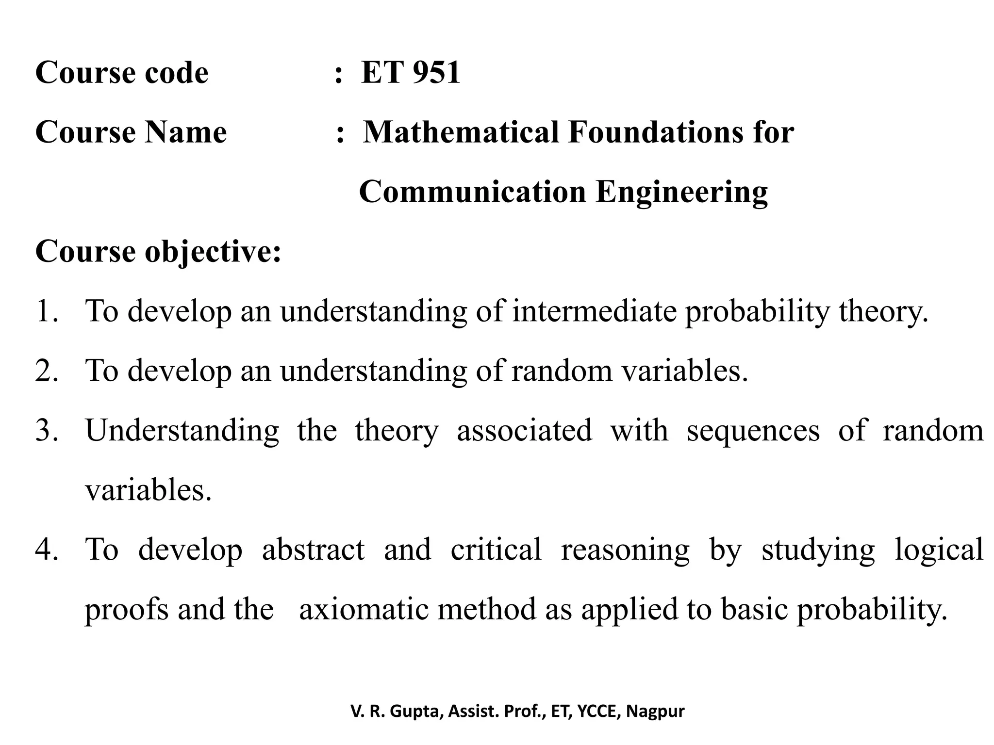
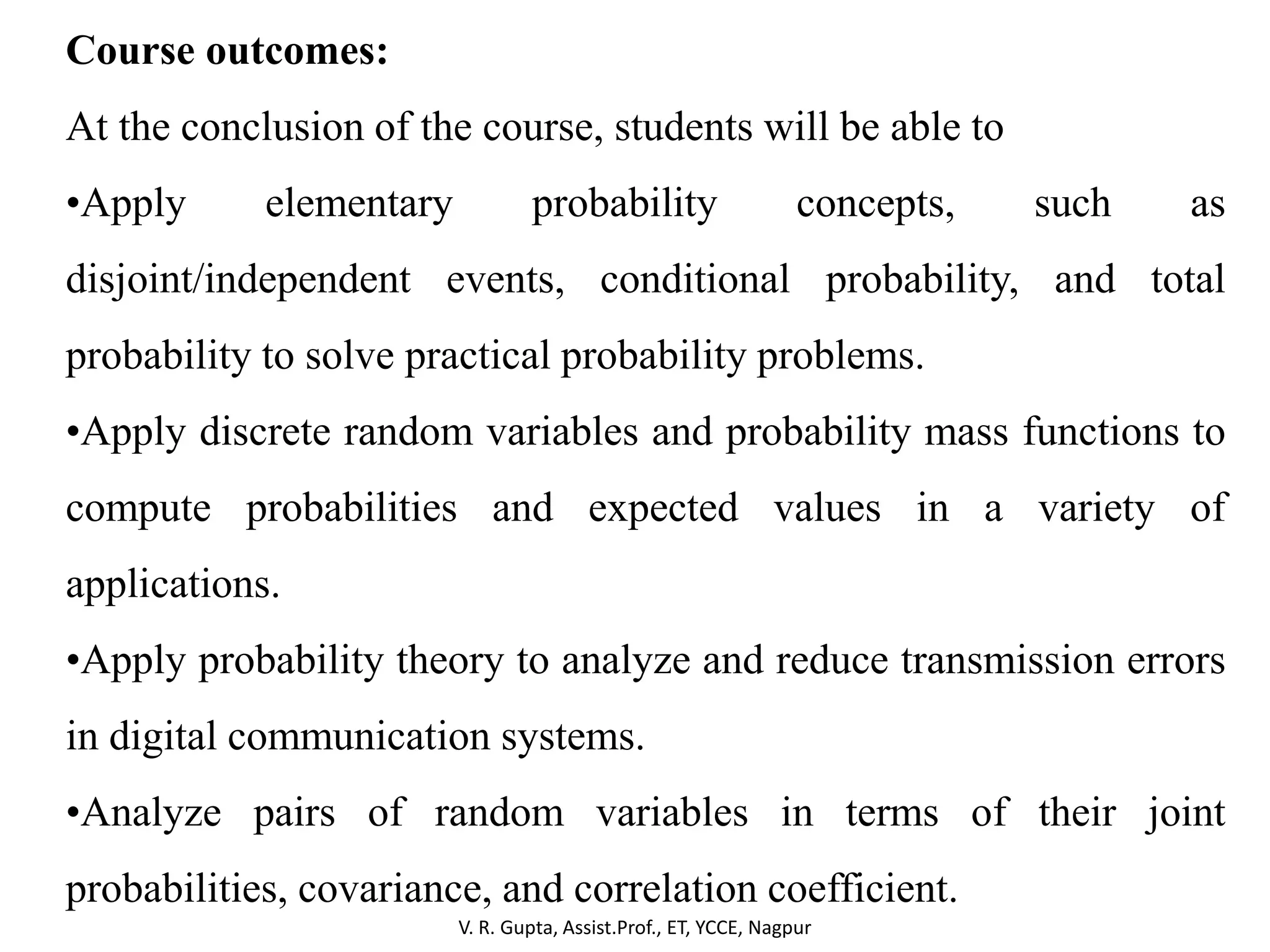
Mathematical Foundation
For
Communication Engineering
V. R. Gupta
Assistant Professor
Department of Electronics and Telecommunication
YCCE, Nagpur

V. R. Gupta, Assist. Prof., ET, YCCE, Nagpur
Course code : ET 951
Course Name : Mathematical Foundations for
Communication Engineering
Course objective:
1. To develop an understanding of intermediate probability theory.
2. To develop an understanding of random variables.
3. Understanding the theory associated with sequences of random
variables.
4. To develop abstract and critical reasoning by studying logical
proofs and the axiomatic method as applied to basic probability.

V. R. Gupta, Assist.Prof., ET, YCCE, Nagpur
Course outcomes:
At the conclusion of the course, students will be able to
•Apply elementary probability concepts, such as
disjoint/independent events, conditional probability, and total
probability to solve practical probability problems.
•Apply discrete random variables and probability mass functions to
compute probabilities and expected values in a variety of
applications.
•Apply probability theory to analyze and reduce transmission errors
in digital communication systems.
•Analyze pairs of random variables in terms of their joint
probabilities, covariance, and correlation coefficient.

•Apply continuous random variables and probability density
functions to compute probabilities and expected values in a variety
of applications.
•Use Matlab to calculate probabilities and simulate the performance
of systems containing randomness.
•Develop probability models and Prove elementary probability
results.
•Perform rigorous probability calculations involving random
variables.
•Obtain distributional information about a random variable.
•Determine the distribution of a functional combination of given
random variables

Course Assessment:
Grading is based on the following components that are weighted
as described below:
 Home Assignments : 5 %
 Open book Test : 2 %
 Quiz : 2 %
 Attendance : 1%
 Mid Sem. Exam-1 : 15%
 Mid Sem. Exam-2 : 15%
 End Sem. Exam. : 60%

UNIT-1: Introduction to Probability :
Definitions, scope and history; limitation of classical and relative-frequency-
based definitions. Sets, fields, sample space and events; axiomatic definition of
probability. Combinatory: Probability on finite sample spaces. Joint and
conditional probabilities, independence, total probability; Bayes’ rule and
applications
UNIT-2: Random variables :
Definition of random variables, continuous and discrete random variables,
cumulative distribution function (cdf) for discrete and continuous random
variables; probability mass function (pmf); probability density functions (pdf)
and properties. Jointly distributed random variables, conditional and joint
density and distribution functions, independence; Bayes’ rule for continuous
and mixed random variables.
UNIT-3: Function of random a variable.
pdf of the function of a random variable; Function of two random variables;
Sum of two independent random variables. Expectation: mean, variance and
moments of a random variable. Joint moments, conditional expectation;
covariance and correlation; independent, uncorrelated and orthogonal random
variables. Random vector: mean vector, covariance matrix and properties.

UNIT-4: Some special distributions:
Uniform, Gaussian and Rayleigh distributions; Binomial, and Poisson
distributions; Multivariate Gaussian distribution
Vector-space representation of random variables, linear independence, inner
product, Schwarz Inequality
Elements of estimation theory: linear minimum mean-square error and
orthogonality principle in estimation; Moment-generating and characteristic
functions and their applications, Bounds and approximations: Chebysev
inequality and Chernoff Bound.
UNIT-5: Sequence of random variables and convergence:
Almost sure (a.s.) convergence and strong law of large numbers; convergence in
mean square sense with examples from parameter estimation; convergence in
probability with examples; convergence in distribution. Central limit theorem
and its significance.
UNIT-6: Random process
Basic definitions, important Random processes, continuous-time linear systems
with random inputs white noise, classification of random processes, WSS
processes and LSI systems.

Assign.
No.
Topic
Date
given
Last Date of
submission
Remark
1. Based on Unit I & II
2. Based on Unit III & IV
3.
Based on Unit V and VI
(Self Learning topic)
Assignments

Text Books:
 “Probability and Random Processes,” by H. Stark, J.W Woods,
Pearson Education, 2000.
 “Probability, Random Variables and Stochastic Processes,” by
A. Papoulis, S. U. Pillai, McGraw Hill, 2002.
Reference Books:
 Probability and Stochastic Processes, by R D Yates, D J
Goodman, John Wiley and Sons, 1992.

Why study probability?

What is probability?
• Mathematical model
• Help us to study physical systems in an
average sense.

Different Kinds of Probability
• Probability as intuition
• Probability as the Ratio of Favorable to Total
Outcomes (Classical Theory)
• Probability as a Measure of Frequency of
Occurrence
• Probability Based on an Axiomatic Theory

Probability as intuition
• Deals with judgments based on intuition.
• Eg: Joe will be wary about letting his nine-
year-old daughter Jane swim in the local pond,
if Frank reports that Bill thought that he might
have seen an alligator in it.

Probability as the Ratio of Favorable to Total
Outcomes (Classical Theory)
• Probability of an event is computed a priori.
• where: NE is the no. of ways E can occur
• N is the no. of all possible outcomes.
• Eg: we throw a pair of unbiased dice and ask what is
the probability of getting a seven?
EN
N

2nd Die
1st Die
1 2 3 4 5 6
1 2 3 4 5 6 7
2 3 4 5 6 7 8
3 4 5 6 7 8 9
4 5 6 7 8 9 10
5 6 7 8 9 10 11
6 7 8 9 10 11 12
The total no of outcomes is 36 if we keep the Dice distinct.
The number of ways of getting a seven is N7 = 6.
6 1
[ 7]
36 6
P getting a  

Probability as a Measure of Frequency of
occurrence
• The Probability of an event E is computed as.
•
• here and therefore
• We can never perform the experiment an infinite number of
times so we can only estimate P[E] from a finite number of
trials.
• We postulate that approaches a limit as n goes to
infinity.
[ ] lim E
n
n
P E
n

En n 0 [ ] 1P E 
En n

Probability Based on an Axiomatic Theory
• Experiment: an experiment is a procedure we perform that
produces some result. Often letter ‘E’ is used to designate an
experiment. (e.g., the experiment E5 might consist of tossing a
coin five times)
• Outcome: An outcome is a possible result of an experiment.
The Greek letter (xi ) is often used to represent outcomes.
(e.g., the outcome of experiment E5 might represent the
sequence of tosses head-head-tail-head-tail; however, the more
concise HHTHT might also be used.)

1

Event: An event is a certain set of outcomes of an experiment.
(e.g., the event C associated with experiment E5 might be C={all
outcomes consisting of an even number of heads}) .
Sample Space: The sample space is the collection of set of “all
possible” distinct (collectively exhaustive and mutually exclusive)
outcomes of an experiment. The letter S is used to designate the
sample space, which is the universal set of outcomes of an
experiments.

• Set: A set is a collection of objects called elements.
E.g., “car, apple, pencil” is a set whose elements are a car, an
apple & a pencil. The set “heads, tails” has two elements.
• The symbol denotes set inclusion and the symbol is the
opposite of .
• How to define a set?
 

{ , , }A RTM University SGB iversity PuneUniversity n
2
{ 1,2,3,.....}B x x 
{ }C all RTM University students whoareinFinalYear BE

• Subset: A subset B of a set A is another set whose elements are
also elements of A.
• Set Equality:
• The definition of set equality is
• Universal set: It is a set of all things that we could possibly
consider in a given context. All set under consideration will be
subsets of a set S, which we shall call space or universal set.
B A
A B
A B iff B A and A B  

• Null set or empty set: By definition the set that contains no
elements is called as Null set or empty set. This is denoted by
{φ}.
S={set of all universities}
• If a set consist of n elements, then the total number of its subsets
equals 2n
.

Set Operations
A B C
C B A or A B C   
, ,
{ }
Thus for any A
A S  

Unions and Intersections
A B or A B U
.
( ) ( )
This operation is comulative and associative
A B B A
A B C A B C


U U
U U U U
A B
, ,
{ }
if B A then A B A
A A A
A A
A S S

 
 


U
U
U
U

Unions and Intersections
AB or A BI
,
.
( ) ( )
( ) )
This operation is comulative
associativeand distributive
AB BA
AB C A BC
A B C AB AC


U U
A B
, ,
{ } { }
if A B then AB A
AA A
A
AS A
 
 
 



Mutually Exclusive Set
{ }AB 
A
B
1 2 3, , .........
{ }i j
several sets A A A are called mutually exclusive if
A A for every i and j i  
Two sets A and B are said to be mutually
exclusive or disjoint if they have no
common elements, that is, if

Partitions
1
1
........ { }
,
,........,[ ]
n i j
n
A A S where A A j i
Thus
A AU
  

U U
A partitions U of a set S is a collection
of mutually exclusive subsets Ai of S
whose union equals S.
A1
A2
An
B

Complements
ĀA
The complement Ā of a set A is the
set consisting of all elements of S
that are not in set A. Thus
{ } { }A A S AA A A S    U
, ;
, ;
if B A then B A
if A B then B A
 
 

Demorgan’s Law
A B AB
AB A B


U
U
AB
AB

If in a set identity we replace all sets by their
complements, all unions by intersections, and all
intersections by unions, the identity is preserved.
( )A B C AB ACU U
( )A B C A B C A BC U U U U
( )( ) ( )( )AB AC AB AC A B A C U U U
( )( )A BC A B A CU U U

Duality Principle
We know that, .
If in an set identity all overbars are removed, the identity
is preserved.
If in a set identity we replace all unions by intersections,
all intersections by unions, and the sets S and {ϕ} by the
sets {ϕ} and S, the identity is preserved.
( )A B C AB AC S A S U U U
{ } { }S and S  
( )( ) { } { }A BC A B A C A  U U U

A BU A BI c
A
A B A B A B

Probability Space
•The space, S or Ω is called the certain event, its
elements experimental outcomes, and its subsets
events.
•The empty set {ϕ} is the impossible event.
•The event {ξ i} consisting of a single element ξ i is an
elementary event .

In the applications of probability theory to physical
problems, the identification of experimental outcomes is
not always unique.

In the relative frequency interpretation of various results, we shall
use the following terminology:
Trial: A single performance of an experiment will be called a trial.
An event A occurs during this trial if it contains the element {ξi}
The certain event occurs at every trial.
The impossible event never occurs.

Axiomatic definition of Probability
Probability is a set function P[.] that assigns to every event E a
number P[E] called the probability of E such that
1. P[E] ≥ 0
2. P[Ω] =1
3. P[E U F]=P[E]+P[F] If EF= ϕ
These conditions are the axioms of the theory of probability

Properties
 The probability of the impossible event is zero.
These conditions are the axioms of the theory of probability
4. [ ] 0
5. [ ] [ ] [ ]
6. [ ] 1 [ ]
7. [ ] [ ] [ ] [ ]
8. [ ] [ ] [ ]
c
c
c
P
P EF P E P EF
P E P E
P E F P E P F P EF
P E P B P AB iff B A
 
 
 
  
  
U

Equality of Events
Two events A and B are called equal if they consist of the same
elements.
c c
AB A BU
They are called equal with probability 1 if the set
consisting of all outcomes that are in A or in B but not in AB
has zero probability. .
c c
AB A BU

Introduction to Probability

More Related Content

What's hot

Similar to Introduction to Probability

More from Vikas Gupta

Recently uploaded

In this document

Introduction to Probability