“Introduction to Modern Radar for Machine Perception,” a Presentation from Sensor Cortek

Introduction to Modern
Radar for Machine
Perception
Robert Laganière
Professor, University of Ottawa
CEO, Sensor Cortek

1. Radar: fundamental principle
2. Radar history and modern radar development
3. Technology for radar: time of flight, continuous wave radar, frequency modulation
4. FMCW radar: the chirp signal, signal mixing
5. FMCW signal processing: range, Doppler, direction of arrival
6. The Range-Azimuth-Doppler signal
7. Detection from radar: constant false alarm rate algorithms
8. Pros and cons of radars
9. Conclusion
Content
2
© 2024 University of Ottawa / Sensor Cortek inc

• Radar is a relatively old technology
• Mature solid-state design, very reliable
• New applications emerged in recent years
• Occupancy detection
• Gesture recognition
• Automotive (ADAS and AV)
• Almost every aspect of radar performance has improved
• Cost, size, power, resolution, etc.
Radar development
3

• 1886-1889, German physicist Heinrich Hertz experimentally
prove the existence of radio waves
• Predicted by Maxwell’s theory of electromagnetism (1865)
• 1904, German engineer Christian Hülsmeyer invented
Telemobiloscope
• First patented device to use radio waves for detecting objects
• 18th May 1904 first public demonstration
• World War II stimulated the development and large-scale
deployment of Radar
Radar history
4
radarworld.org/huelsmeyer.html

1. Time of Flight (ToF)
2. Continuous Waves (CW)
3. Frequency Modulation (FM)
 FMCW Radar
Three technologies for radar
5
https://hforsten.com/third-version-of-homemade-6-ghz-fmcw-radar.html

• In its simplest form, an impulse signal is sent
• Measuring time to receive the echo yield to distance estimate according to:
1. Time of flight (ToF) for distance estimation
6
www.radartutorial.eu/01.basics/Distance-determination.en.html
monostatic
radar

• The power received Pr is a fraction of the power transmitted Pt
• σ is the radar cross section (expressed in m2) defines how detectable is the target; it
depends on:
• Target material
• Target shape
• Target size
• Incident angle
Radar cross section
7
Pt
Pr
Pr= Pt x (gain) x (spread factor) x (losses) x σ x (spread factor) x (aperture) x (dwell time)

• A continuous signal is transmitted
• The Doppler effect provides target velocity information
• The Doppler frequency is the difference between the transmitted signal frequency
and the received signal frequency
2. Continuous wave (CW) and the Doppler effect
8
copradar.com/chapts/chapt3/ch3d1.html

• Technique for encoding of information
into a wave signal by varying its
instantaneous frequency
• For radar this is a way to add information
• To better estimate velocity and range via
Doppler shift
• To reduce interference by making the
signal more distinctive
3. Frequency modulation (FM) signal encoding
9

• FMCW radars transmit and receive a signal that combine FM and CW techniques
• The signal frequency changes periodically w.r.t time, one period is often referred to as
one “chirp”
FMCW signal
10
• Signal parameters:
• Chirp periodicity Tc;
• Frequency slope S;
• Frequency bandwidth of one chirp B.
• As we will see, the choice of the signal
parameters will affect the radar performance
• A radar frame is made of N chirps

• The transmitted (Tx) and received (Rx) signals are mixed by an onboard mixer
• The resulting signal is then digitized by an analog to digital converter (ADC)
FMCW signal mixing
11

• The frequency difference fb between the Tx and Rx signals is called the beat frequency
• The beat frequency carries range and velocity information
• The frequency shift (or Doppler shift) fd is proportional to velocity
• The time shift τ is proportional to the distance of the target
The mixed signal
12
uwaterloo.ca/centre-for-intelligent-antenna-and-
radio-systems/sites/ca.centre-for-intelligent-
antenna-and-radio-
systems/files/uploads/files/fmcwradarsystem.pdf

• The input signal is a radar frame composed of N Chirps
• This is the ADC signal
• i.e., the signal from the Analog-to-Digital converter
• The Fast Fourier Transform (FFT) is the main tool for the analysis of FMCW radars
• Traditional FMCW DSP is normally divided into 3 steps:
• Range FFT
• Doppler FFT
• Direction of Arrival (DOA)
• The resulting signal is three-dimensional and is therefore designated as the:
• Radar Data Cube
FMCW digital signal processing
13

• The beat frequency fd (a.k.a. intermediate
frequency) is computed by FFT from ADC signals.
• The theoretical maximum range is limited by the
chirp periodicity (τ < Tm).
• In practice it is limited by the power of the signal
and the ADC sampling rate.
• To increase the range resolution, you must
increase the chirp frequency bandwidth B.
• This range FFT is conducted with the signals
collected in one chirp.
The range FFT
14
uwaterloo.ca/centre-for-intelligent-antenna-and-
radio-systems/sites/ca.centre-for-intelligent-
antenna-and-radio-
systems/files/uploads/files/fmcwradarsystem.pdf

• The velocity is extracted by
observing the change in
phase of the beat frequency
between consecutive chirps.
• This Doppler FFT is therefore
computed over the series of
chirps in a radar frame.
• To increase the range
resolution, you must increase
the number of chirps in the
radar frame.
Doppler FFT
15

Range and velocity estimation summary
16
Definition:
Resolution:
Maximum:
c, Speed of light
IFtone, Beat frequency
S, Chirp frequency slope
Tc, Chirp period
D, Chirp frequency bandwidth
Tf, Frame period
Fs, ADC sampling frequency

• MIMO radars use multiple transmitting (Tx) and receiving (Rx) antennas
• Creating (Tx) x (Rx) virtual antennas (i.e. mixed signals)
• The angle estimation is based on the phase differences between the signals
received from different onboard receivers.
• Signals transmitted from different transmitters and received at different
receivers are rearranged into an array called Virtual Antennas.
• Based on the physical arrangement of the
antennas, you can measure both
• Vertical (Elevation) and
• Horizontal (Azimuth) directions
• 3Tx and 4Rx antennas = 12 channels is a common configuration
Direction of arrival (MIMO)
17
www.ti.com/lit/an/swra554a/swra554a.pdf?ts=1616040203534

• The ADC signal is pre-arranged into a 3D tensor
• Number of digital samples per chirp X
number of chirps X
number of virtual antennas.
• The output from 3D-FFT is called range-
azimuth-Doppler (RAD) tensor
• The RAD Cube
Range-Azimuth-Doppler: the RAD cube
18
www.semanticscholar.org/paper/79-GHz-wideband-fast-chirp-
automotive-radar-sensor-Sturm-
Li/3d0fb8b52e40bf870bccc908217065ec7a15311a/figure/1

• Range-azimuth-Doppler (RAD) tensors are
usually projected onto 2D planes for
visualization.
• The two most practical planes for visualizing
RAD tensors are:
• Range-Doppler (RD) spectrum
• Range-Azimuth (RA) spectrum
Range-Azimuth-Doppler: the RAD cube
19
Range vs
Velocity
Range vs
Angle

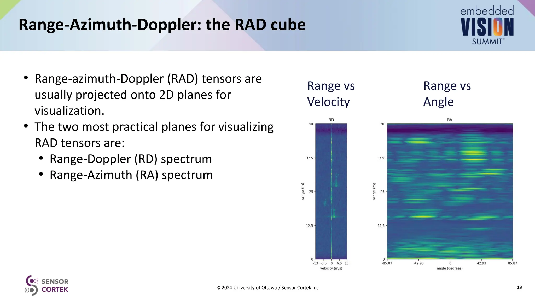
• RA spectrum is presented with [range, angle] representations in polar coordinates.
• To increase the readability, RA data can also be transformed into top-view coordinates.
Polar to Cartesian
20
Range vs
Angle
Cartesian coordinates [X,Z]

• From the information embedded in the RAD cube, it is possible to detect objects.
• But this signal is complex to analyze.
The next step is generally to perform thresholding and clustering operations to extract
meaningful objects.
• The main algorithm to accomplish this objective is the CFAR.
Detection from radar
21

• Constant false alarm rate (CFAR) is the most popular
denoise algorithm for FMCW radars.
• Usually used for the detections on RD spectrum.
• It is a sliding window-based algorithm.
• Different thresholding variants exist:
• Cell averaging: CA-CFAR
• Ordered statistics: OS-CFAR
Constant false alarm rate (CFAR) algorithm
22
www.researchgate.net/figure/Basic-monodimensional-Constant-False-Alarm-
Rate-CFAR-architecture_fig4_343272863
www.radartutorial.eu/01.basics/False%20Alarm%20Rate.en.html
CUT: Cell under test
G: Guard cells
R: Reference cells

Traditional radar pipeline
23
ADC FFT CFAR Thresholding Clustering
FFT
FFT
Point cloud/
object tracking
This is the radar point cloud
before clustering (top-view)
Range-Doppler Range-Azimuth

• Weather-proof:
• FMCW radars can penetrate mediums such as clouds, fogs, mist and snow
• Illumination-proof:
• The signal frequency is specially designed and not affected by other visible light
sources
• Rich detection:
• FMCW radars can detect the positions and speeds of the targeted objects
simultaneously
• Large Field of View (FoV):
• The FoV of FMCW radars is approximately 180 degrees
• Economically friendly:
• FMCW radars are normally cheaper than other sensors in autonomous driving.
Pros of FMCW radars
24

• Noisy:
• The noisy signals lead to difficulties of distinguishing target objects from background
noise
• Unintuitive representations:
• The detection outputs are not visually intuitive to human observers
• Ignorance of some objects:
• Because FMCW radars can penetrate certain materials such as glasses, those objects
are sometimes not visible in radar frames
• No visual details:
• Radars cannot reveal the details of different objects, such as colors, surface
properties, etc.
• For example, it cannot read road signs
Cons of FMCW radars
25

• Radars are cheap, reliable, robust solid-state sensors
• Its claimed robustness to adverse weather condition is assumed but still must be fully
demonstrated
• Radars are becoming an essential component of complex perception systems
• e.g., autonomous vehicles
• Radars are improving in resolution and accuracy
• Deep neural networks (artificial intelligence) can be applied to radar
• Multi-sensor integration is the future of perception
• Radars will be part of it
Conclusion
26

References
27
Publications on radar:
• MIMO Radar, Application Report, Texas Instruments, May 2017.
• Automotive FMCW Radar Development and Verification Methods, Master’s thesis, Sanoal Machado Santiago
Manchego, University of Gothenburg, 2018.
• FMCW Radar System, Mostafa Alizadeh, University of Waterloo, 2019
• RADDet: Range-Azimuth-Doppler based Radar Object Detection for Dynamic Road Users, Ao Zhang, F. Nowruzi,
R. Laganière, CRV2021
• T-FFTRadNet: Object Detection with Swin Vision Transformers from Raw ADC Radar Signals, Giroux, Bouchard,
Laganiere, IEEE/CVF International Conference on Computer Vision Workshops, 2023

“Introduction to Modern Radar for Machine Perception,” a Presentation from Sensor Cortek

More Related Content

Similar to “Introduction to Modern Radar for Machine Perception,” a Presentation from Sensor Cortek

More from Edge AI and Vision Alliance

Recently uploaded

“Introduction to Modern Radar for Machine Perception,” a Presentation from Sensor Cortek