The document discusses mediation analysis in health research, focusing on how predictor variables impact outcomes through mediators, illustrated by framework examples like impulsivity affecting binge drinking. It elaborates on statistical methods for testing mediation effects, including linear regression, Sobel tests, and the bootstrapping technique for significance assessment. Additionally, it provides practical guidance on conducting these analyses using SPSS, including effect size calculations and interpreting results.

1. Mediation in health research:
A statistics workshop using SPSS
Dr. Sean P. Mackinnon
Dalhousie University
Crossroads Interdisciplinary Health Conference, 2015

2. What kinds of questions does
mediation answer?
• Mediation asks about the process by which a
predictor variable affects an outcome
• “Does X predict M, which in turn predicts Y?”
• E.g., “Does exercise improve cardiovascular
health, which in turn increases longevity?”

3. Linear Regression
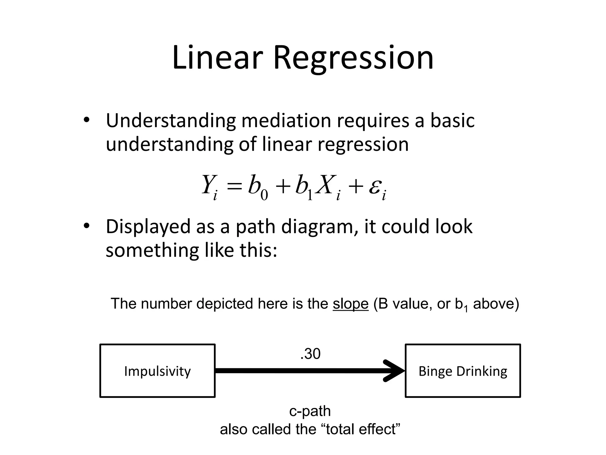
• Understanding mediation requires a basic
understanding of linear regression
• Displayed as a path diagram, it could look
something like this:
Impulsivity Binge Drinking
.30
The number depicted here is the slope (B value, or b1 above)
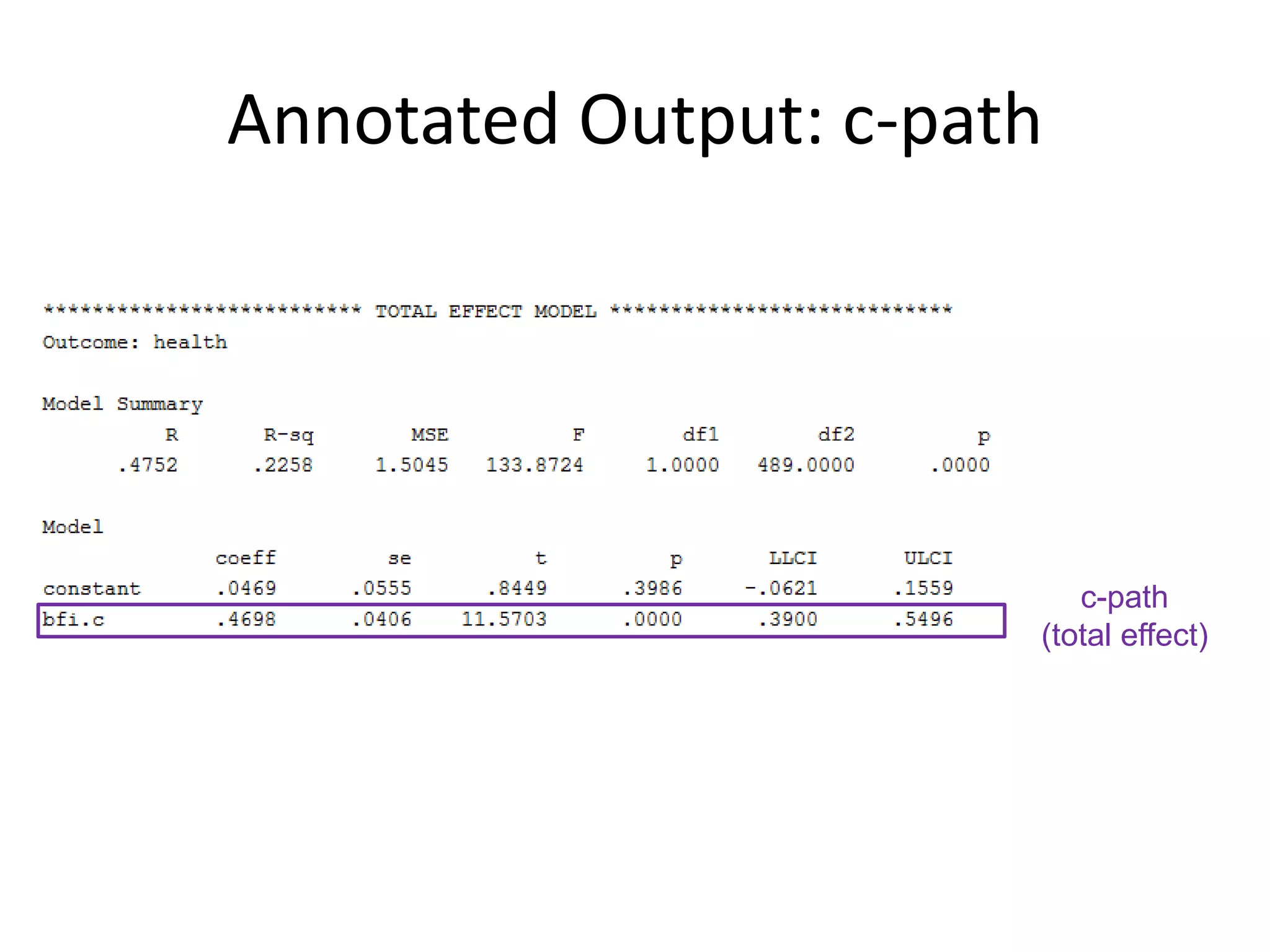
c-path
also called the “total effect”
iii XbbY  10

4. Mediation
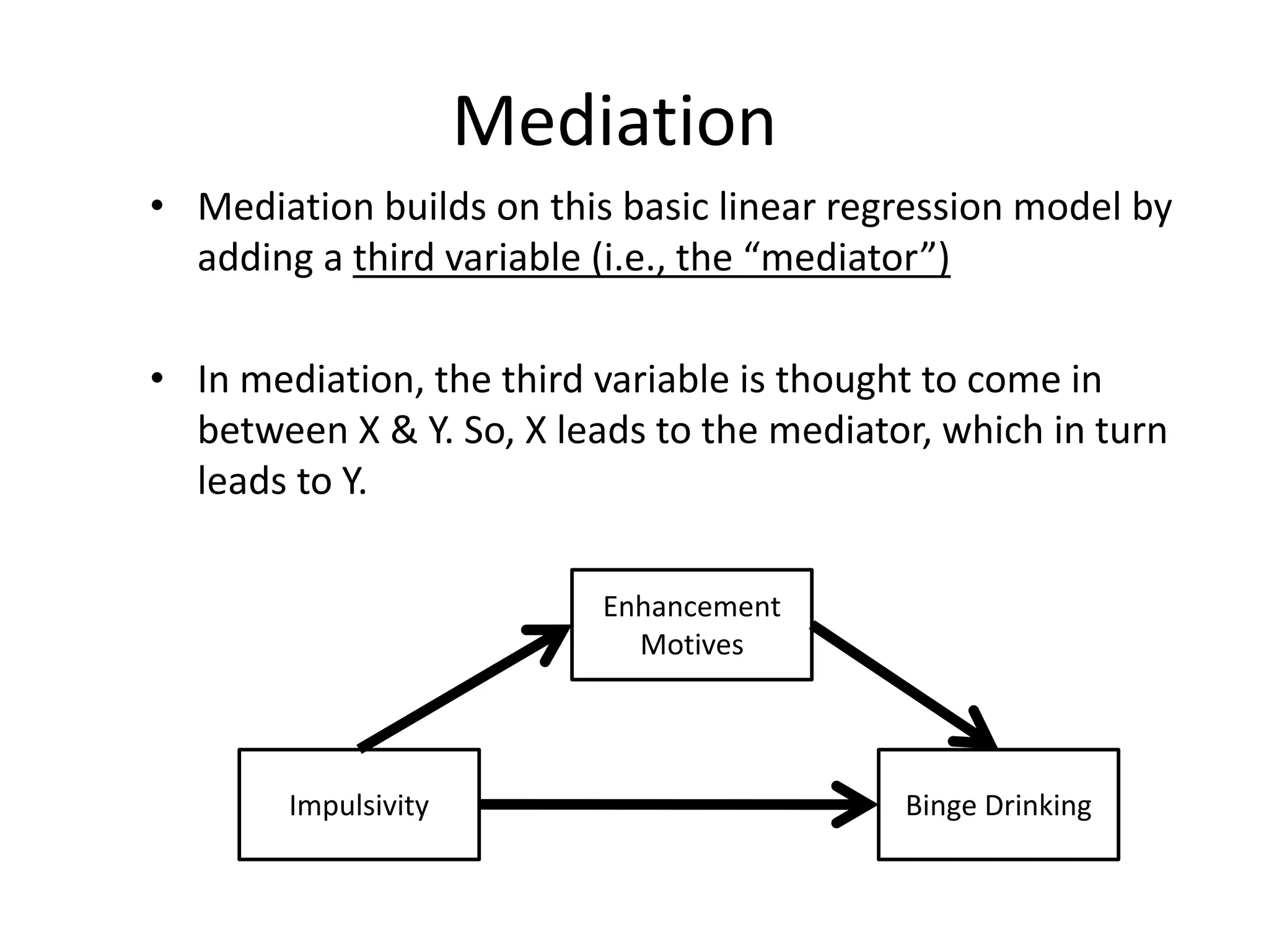
• Mediation builds on this basic linear regression model by
adding a third variable (i.e., the “mediator”)
• In mediation, the third variable is thought to come in
between X & Y. So, X leads to the mediator, which in turn
leads to Y.
Impulsivity Binge Drinking
Enhancement
Motives

5. Mediation
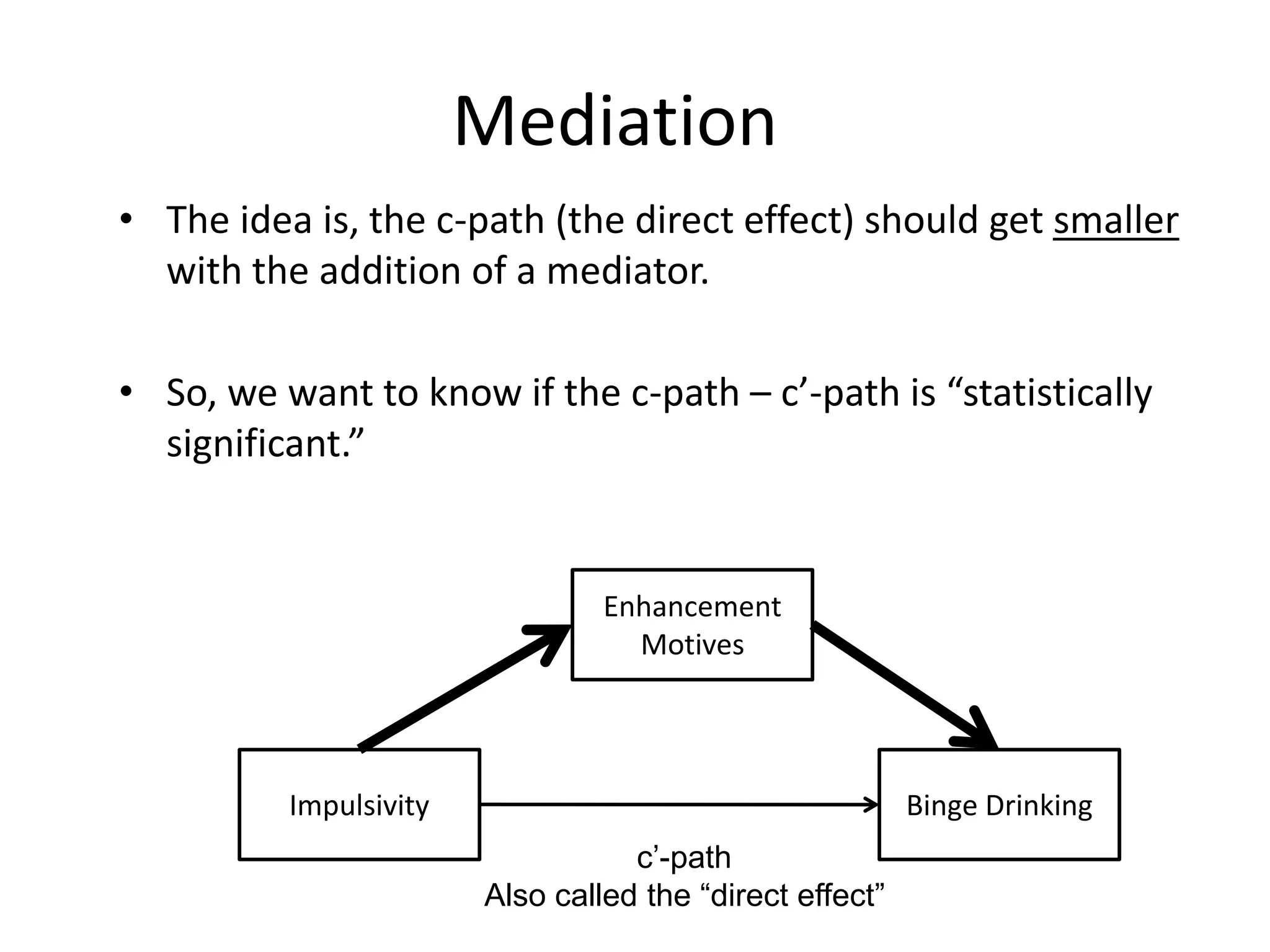
• The idea is, the c-path (the direct effect) should get smaller
with the addition of a mediator.
• So, we want to know if the c-path – c’-path is “statistically
significant.”
Impulsivity Binge Drinking
Enhancement
Motives
c’-path
Also called the “direct effect”

6. Mediation
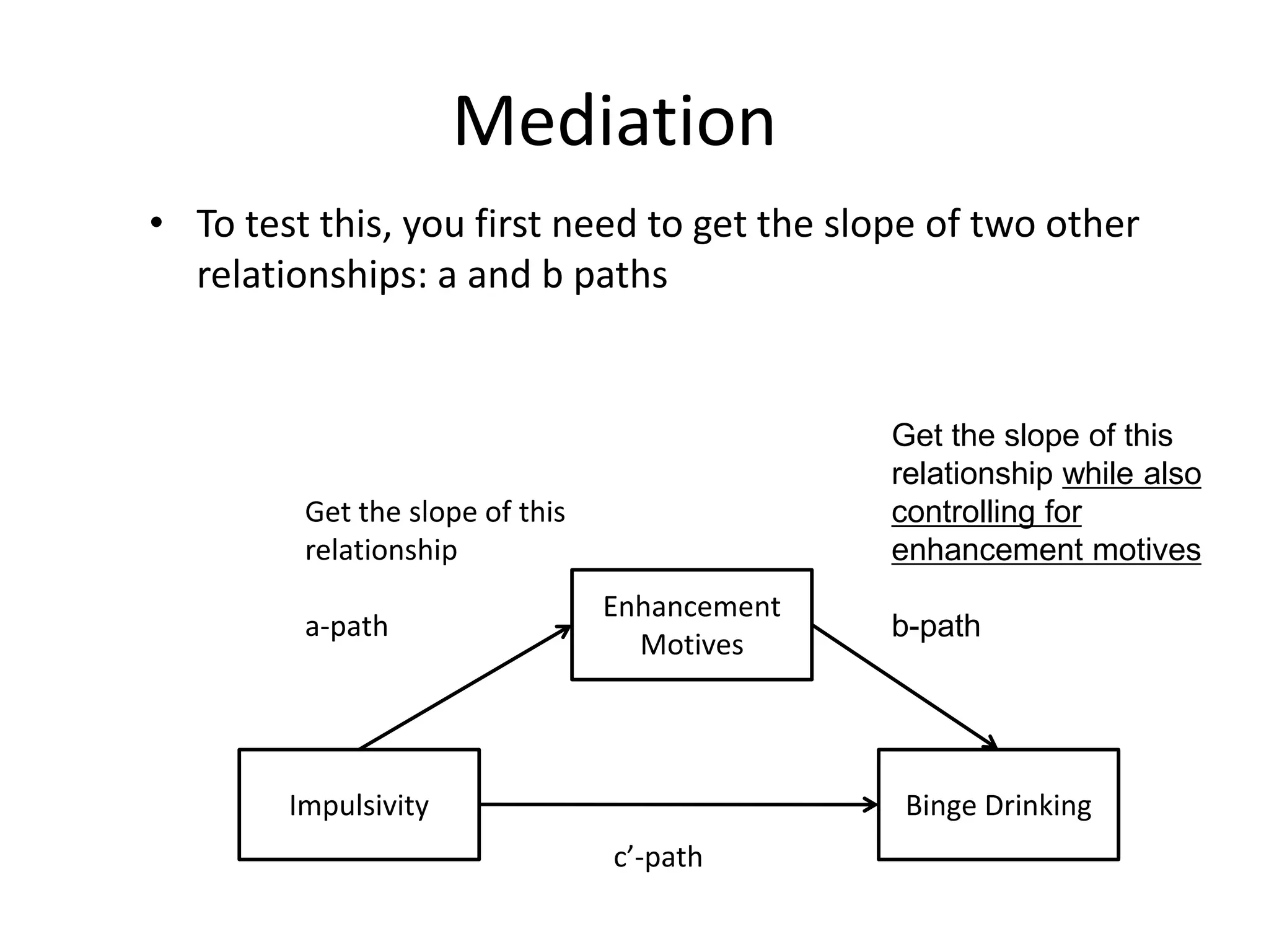
• To test this, you first need to get the slope of two other
relationships: a and b paths
Impulsivity Binge Drinking
Enhancement
Motives
c’-path
Get the slope of this
relationship
a-path
Get the slope of this
relationship while also
controlling for
enhancement motives
b-path

7. Mediation
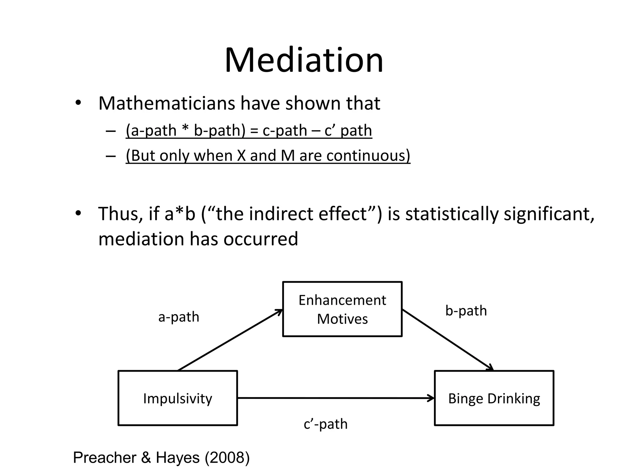
• Mathematicians have shown that
– (a-path * b-path) = c-path – c’ path
– (But only when X and M are continuous)
• Thus, if a*b (“the indirect effect”) is statistically significant,
mediation has occurred
Impulsivity Binge Drinking
Enhancement
Motives
c’-path
a-path b-path
Preacher & Hayes (2008)

8. Significance of Indirect Effect
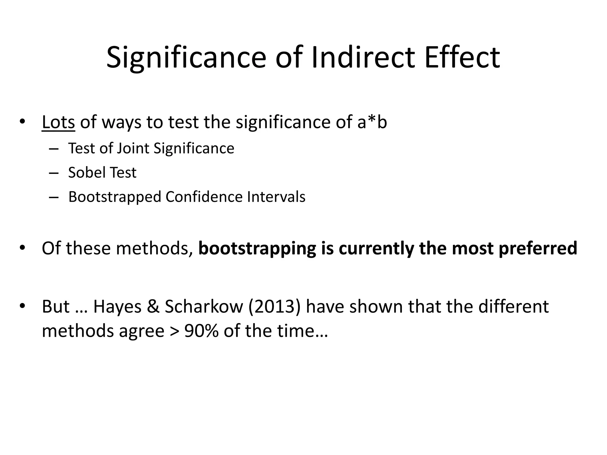
• Lots of ways to test the significance of a*b
– Test of Joint Significance
– Sobel Test
– Bootstrapped Confidence Intervals
• Of these methods, bootstrapping is currently the most preferred
• But … Hayes & Scharkow (2013) have shown that the different
methods agree > 90% of the time…

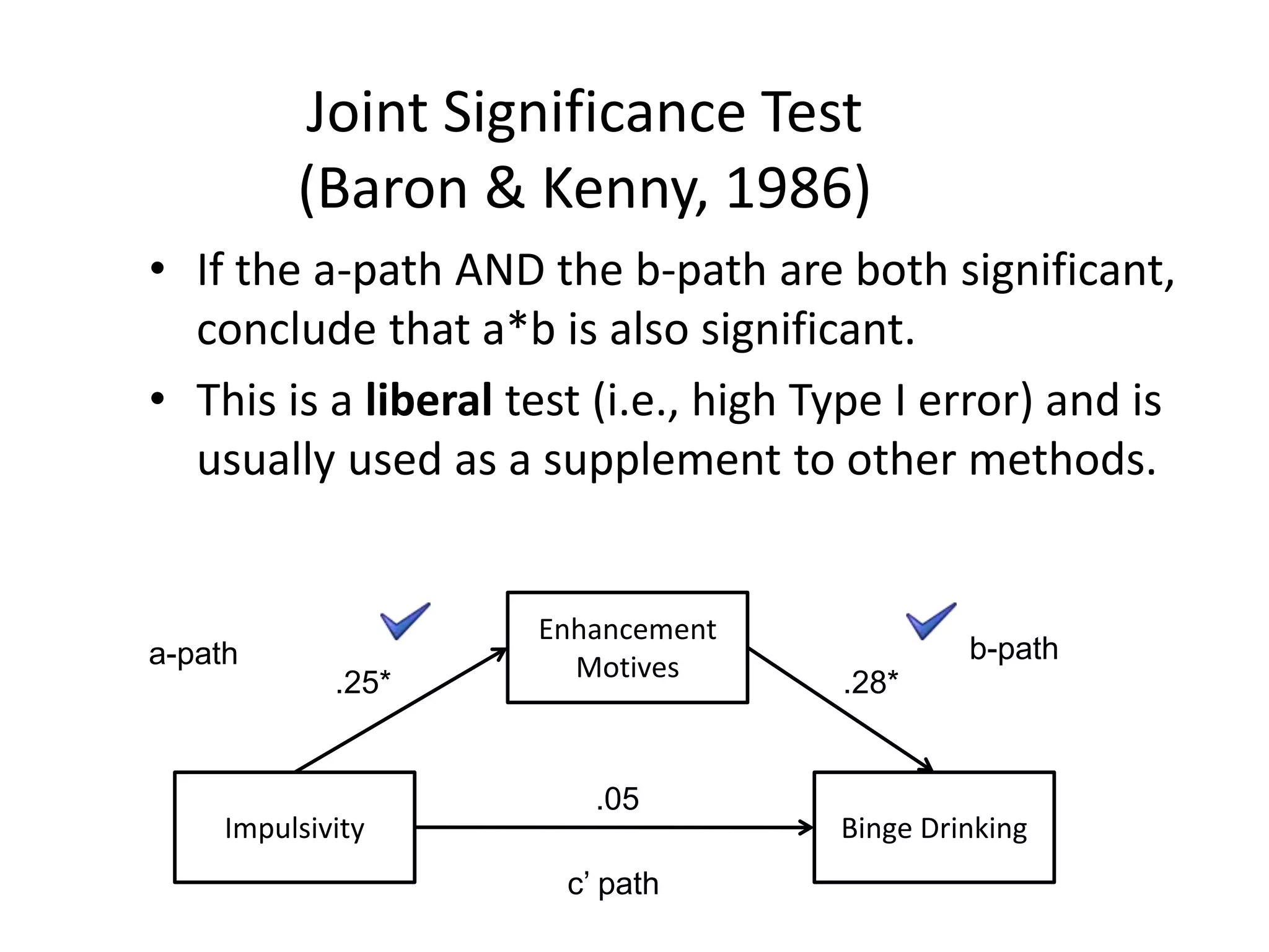
9. Joint Significance Test
(Baron & Kenny, 1986)
• If the a-path AND the b-path are both significant,
conclude that a*b is also significant.
• This is a liberal test (i.e., high Type I error) and is
usually used as a supplement to other methods.
Impulsivity Binge Drinking
Enhancement
Motives
.05
.25* .28*
c’ path
a-path b-path

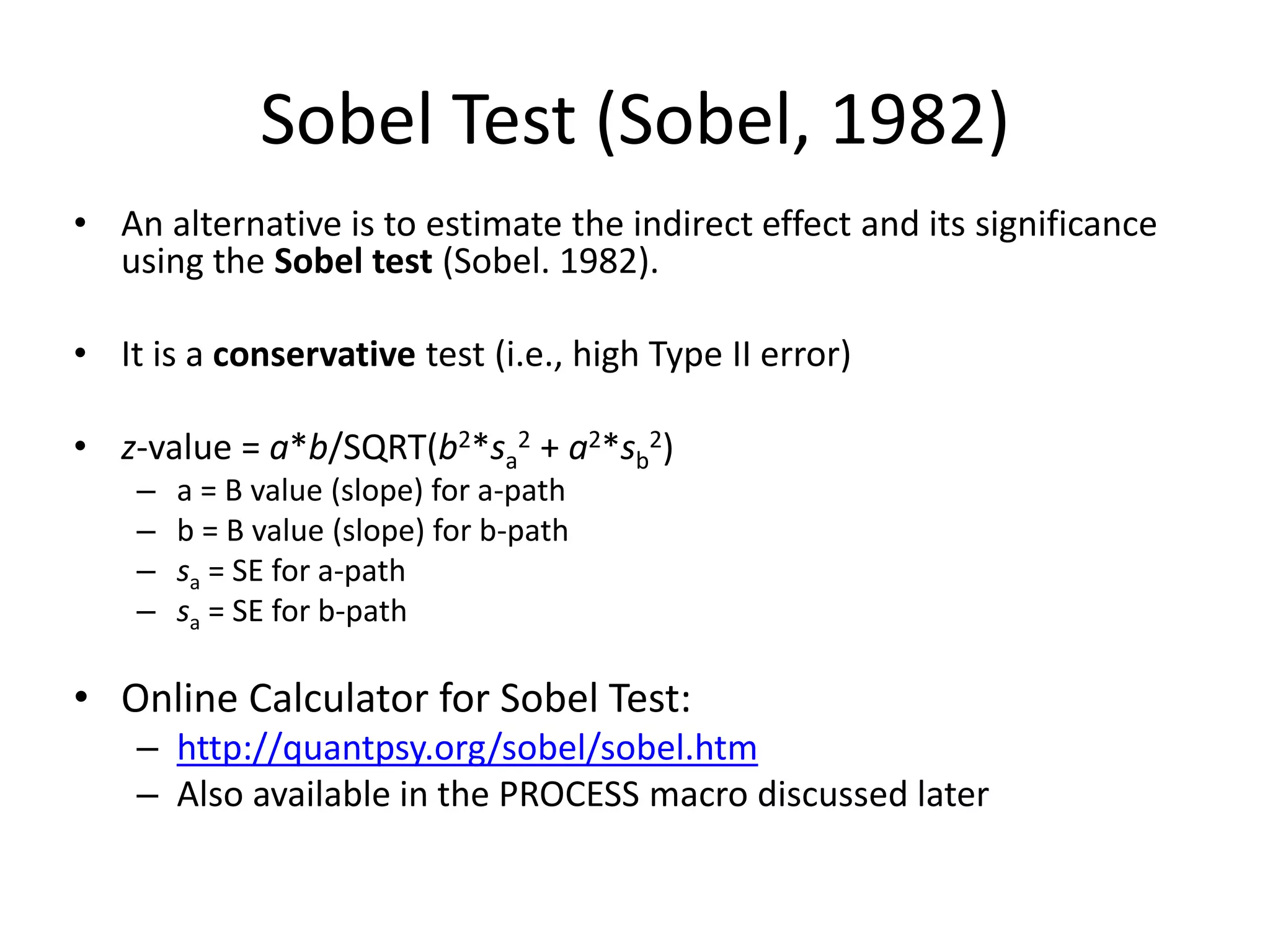
10. Sobel Test (Sobel, 1982)
• An alternative is to estimate the indirect effect and its significance
using the Sobel test (Sobel. 1982).
• It is a conservative test (i.e., high Type II error)
• z-value = a*b/SQRT(b2*sa
2 + a2*sb
2)
– a = B value (slope) for a-path
– b = B value (slope) for b-path
– sa = SE for a-path
– sa = SE for b-path
• Online Calculator for Sobel Test:
– http://quantpsy.org/sobel/sobel.htm
– Also available in the PROCESS macro discussed later

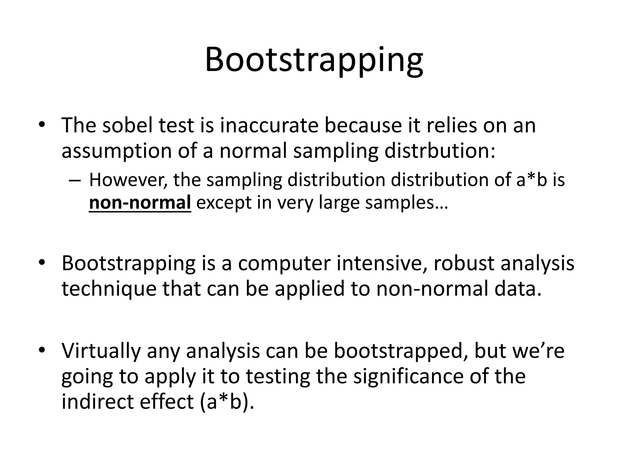
11. Bootstrapping
• The sobel test is inaccurate because it relies on an
assumption of a normal sampling distrbution:
– However, the sampling distribution distribution of a*b is
non-normal except in very large samples…
• Bootstrapping is a computer intensive, robust analysis
technique that can be applied to non-normal data.
• Virtually any analysis can be bootstrapped, but we’re
going to apply it to testing the significance of the
indirect effect (a*b).

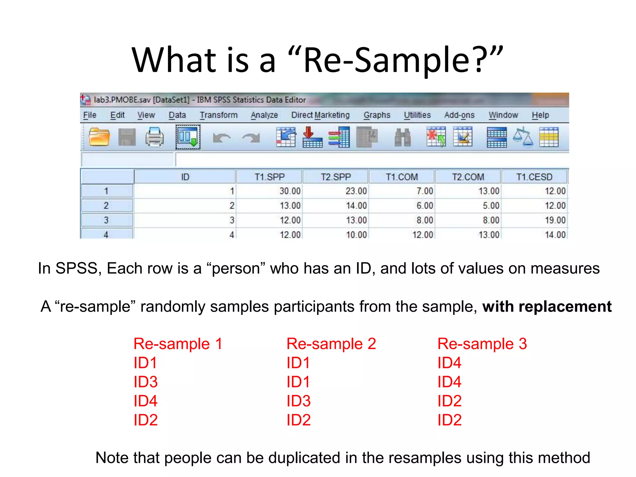
12. What is a “Re-Sample?”
In SPSS, Each row is a “person” who has an ID, and lots of values on measures
A “re-sample” randomly samples participants from the sample, with replacement
Re-sample 1
ID1
ID3
ID4
ID2
Re-sample 2
ID1
ID1
ID3
ID2
Re-sample 3
ID4
ID4
ID2
ID2
Note that people can be duplicated in the resamples using this method

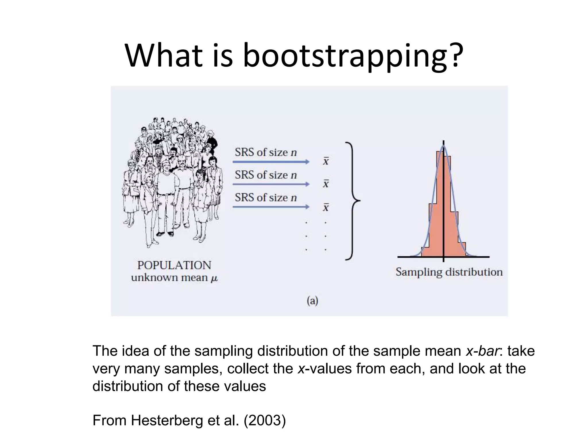
13. What is bootstrapping?
The idea of the sampling distribution of the sample mean x-bar: take
very many samples, collect the x-values from each, and look at the
distribution of these values
From Hesterberg et al. (2003)

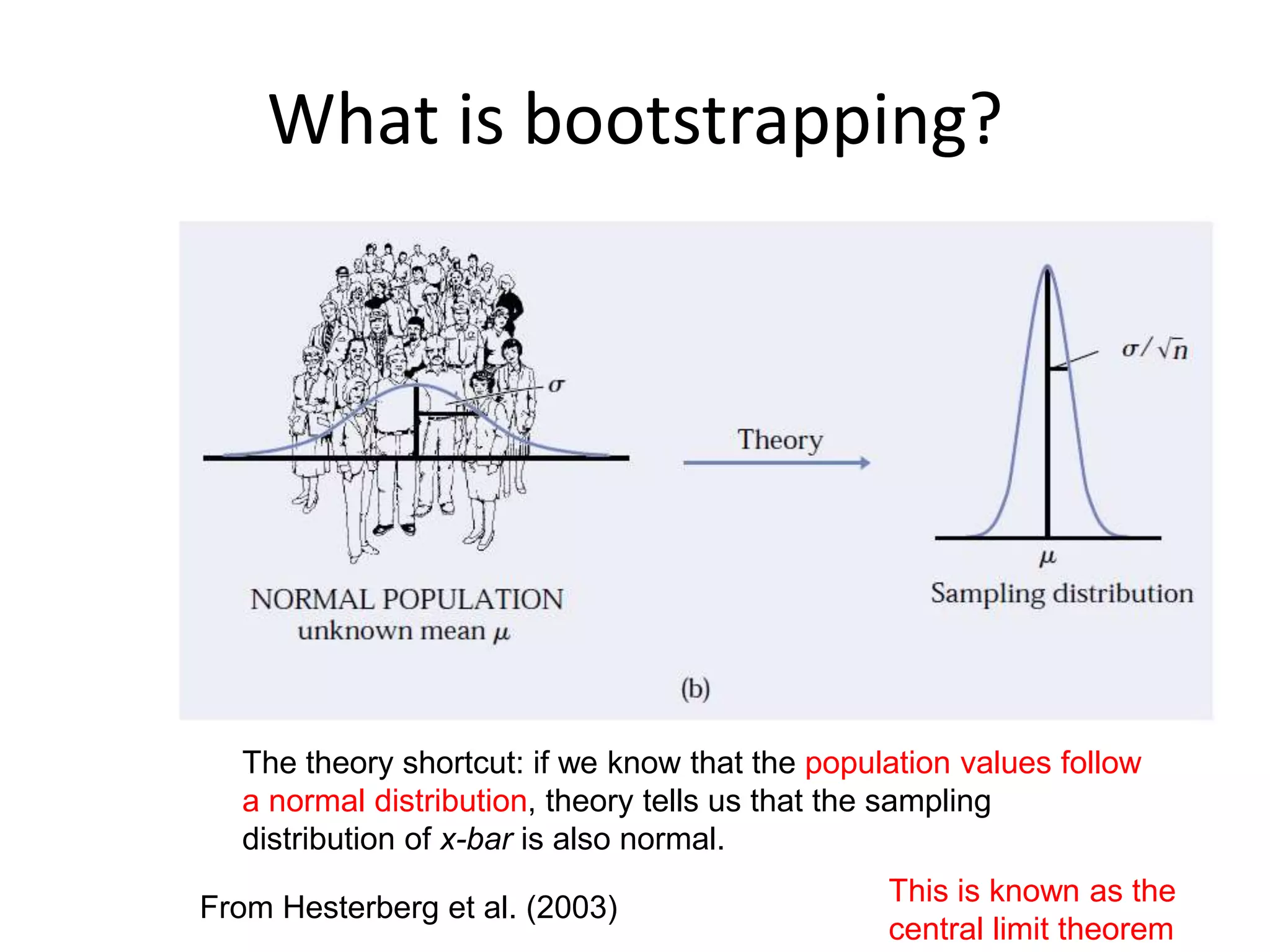
14. What is bootstrapping?
From Hesterberg et al. (2003)
The theory shortcut: if we know that the population values follow
a normal distribution, theory tells us that the sampling
distribution of x-bar is also normal.
This is known as the
central limit theorem

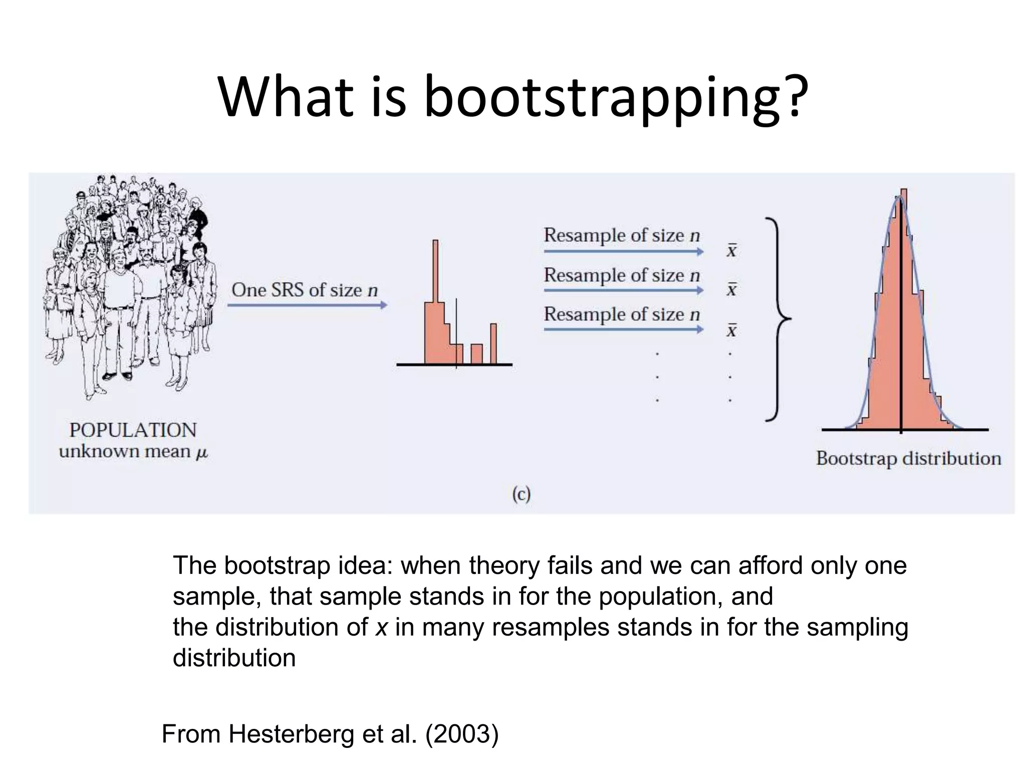
15. What is bootstrapping?
From Hesterberg et al. (2003)
The bootstrap idea: when theory fails and we can afford only one
sample, that sample stands in for the population, and
the distribution of x in many resamples stands in for the sampling
distribution

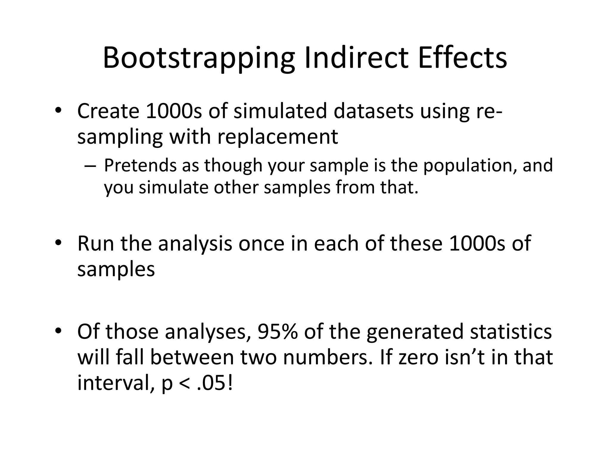
16. Bootstrapping Indirect Effects
• Create 1000s of simulated datasets using re-
sampling with replacement
– Pretends as though your sample is the population, and
you simulate other samples from that.
• Run the analysis once in each of these 1000s of
samples
• Of those analyses, 95% of the generated statistics
will fall between two numbers. If zero isn’t in that
interval, p < .05!

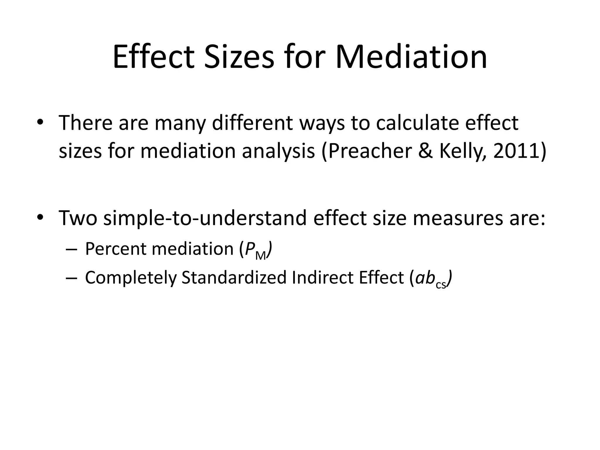
17. Effect Sizes for Mediation
• There are many different ways to calculate effect
sizes for mediation analysis (Preacher & Kelly, 2011)
• Two simple-to-understand effect size measures are:
– Percent mediation (PM)
– Completely Standardized Indirect Effect (abcs)

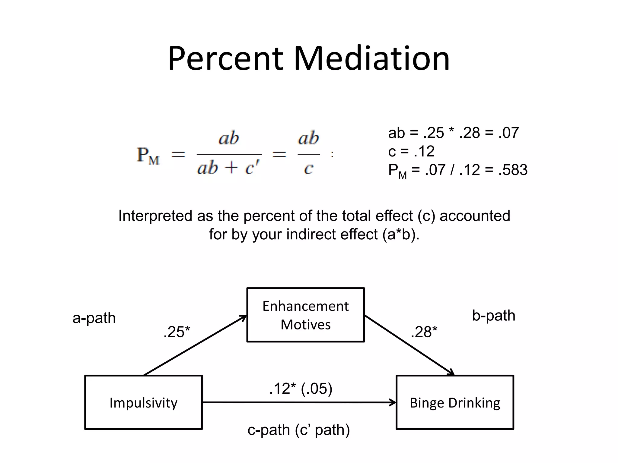
18. Percent Mediation
Impulsivity Binge Drinking
Enhancement
Motives
.12* (.05)
.25* .28*
c-path (c’ path)
a-path b-path
ab = .25 * .28 = .07
c = .12
PM = .07 / .12 = .583
Interpreted as the percent of the total effect (c) accounted
for by your indirect effect (a*b).

19. Note about Percent Mediation…
• The direct effect (c’-path) can sometimes be
larger than the total effect (c-path)
– Inconsistent mediation
• In these cases, take the absolute value of c’
before calculating effect size to avoid
proportions greater than 1.0.

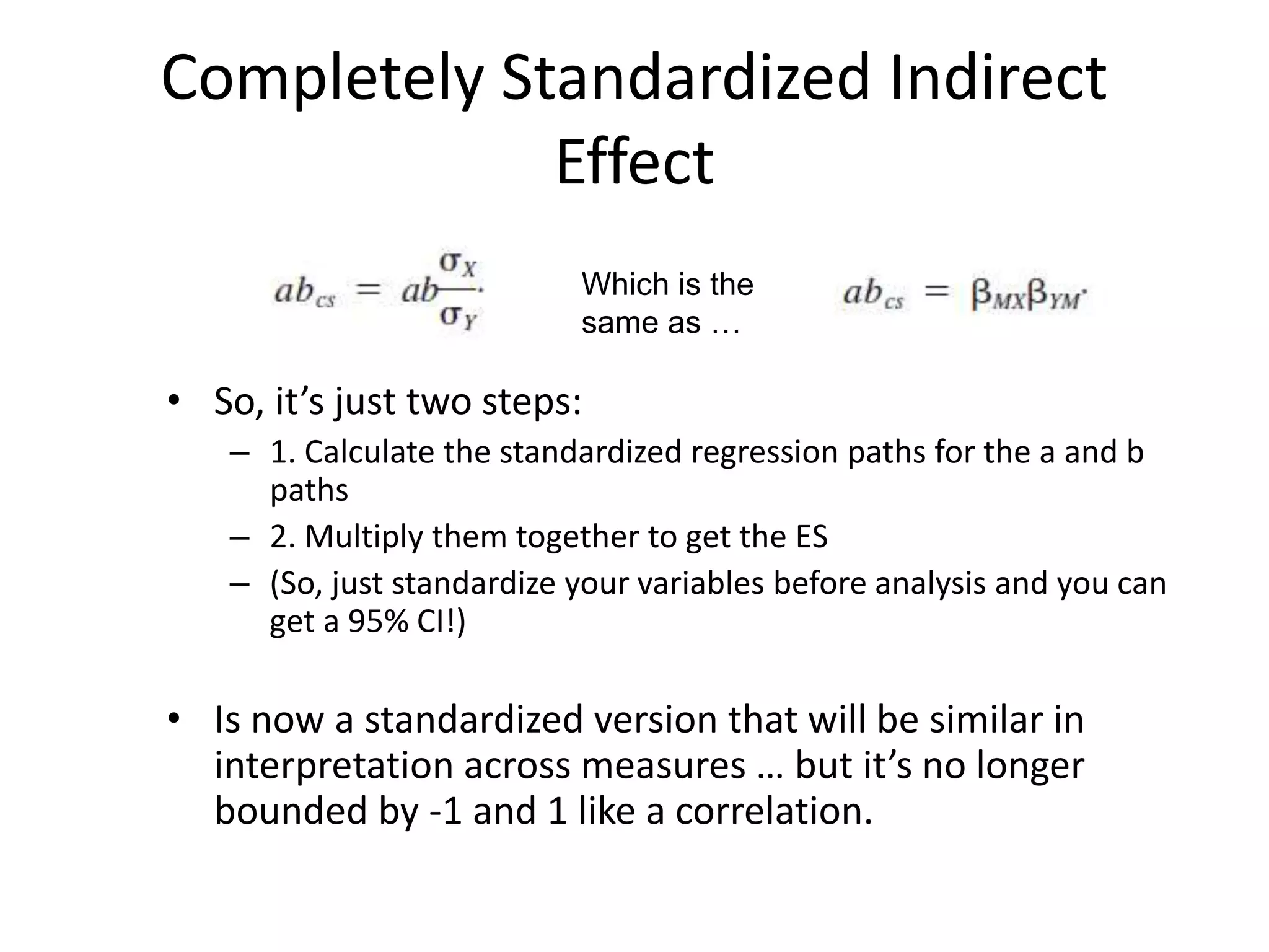
20. Completely Standardized Indirect
Effect
• So, it’s just two steps:
– 1. Calculate the standardized regression paths for the a and b
paths
– 2. Multiply them together to get the ES
– (So, just standardize your variables before analysis and you can
get a 95% CI!)
• Is now a standardized version that will be similar in
interpretation across measures … but it’s no longer
bounded by -1 and 1 like a correlation.
Which is the
same as …

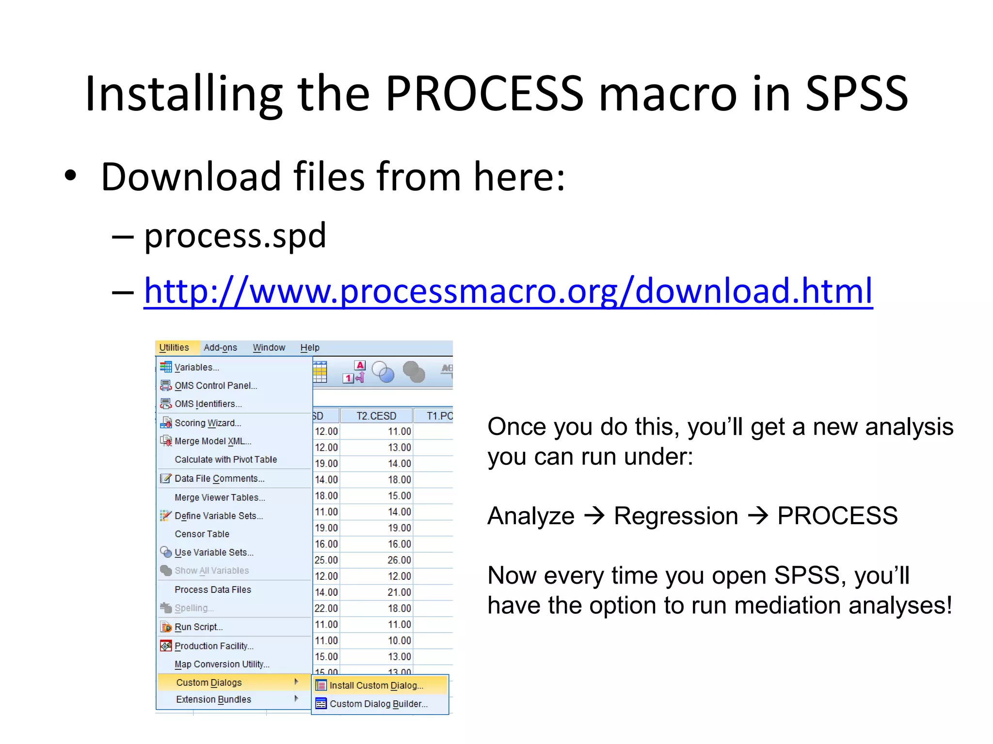
21. Installing the PROCESS macro in SPSS
• Download files from here:
– process.spd
– http://www.processmacro.org/download.html
Once you do this, you’ll get a new analysis
you can run under:
Analyze  Regression  PROCESS
Now every time you open SPSS, you’ll
have the option to run mediation analyses!

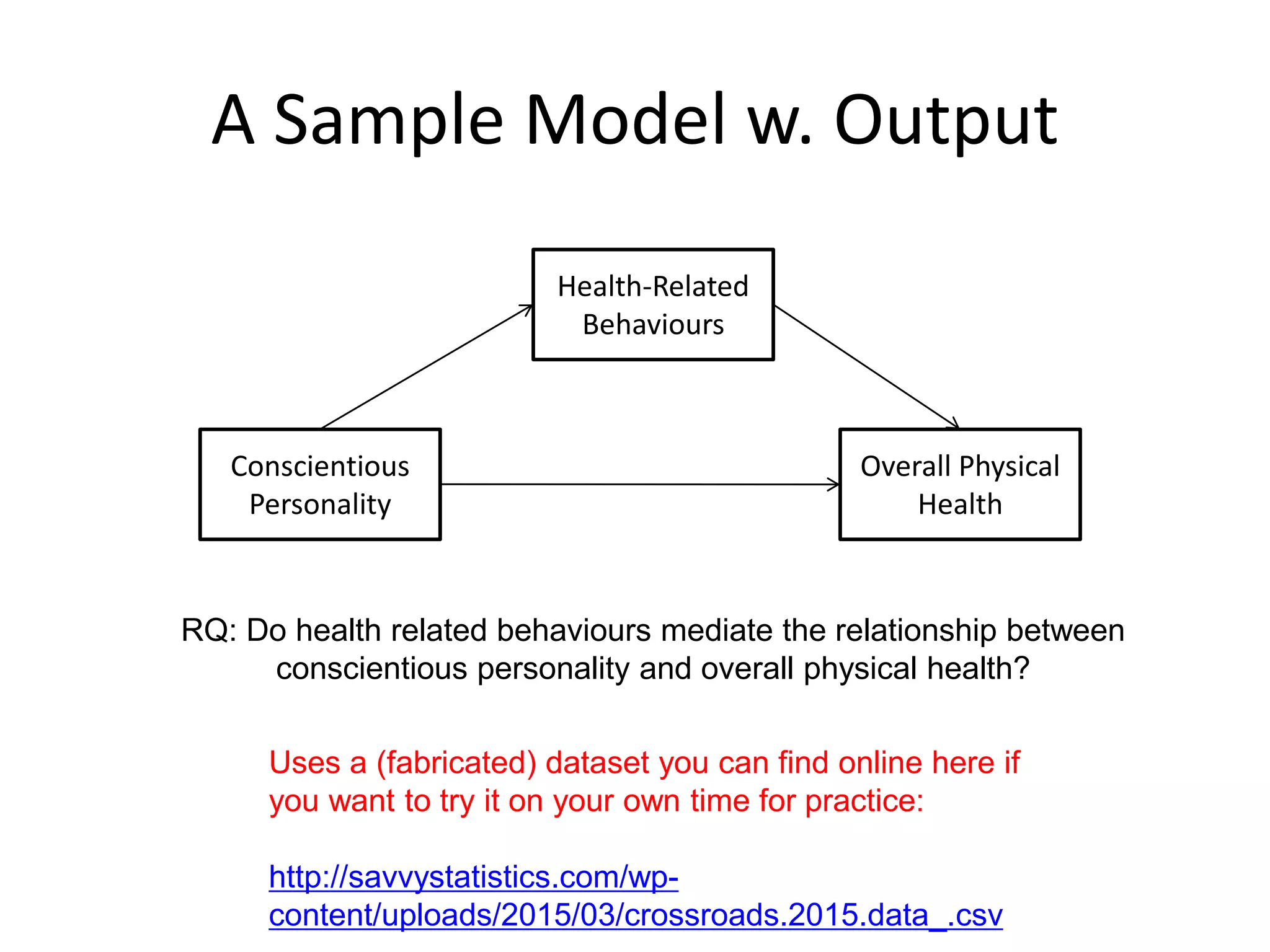
22. A Sample Model w. Output
Conscientious
Personality
Overall Physical
Health
Health-Related
Behaviours
Uses a (fabricated) dataset you can find online here if
you want to try it on your own time for practice:
http://savvystatistics.com/wp-
content/uploads/2015/03/crossroads.2015.data_.csv
RQ: Do health related behaviours mediate the relationship between
conscientious personality and overall physical health?

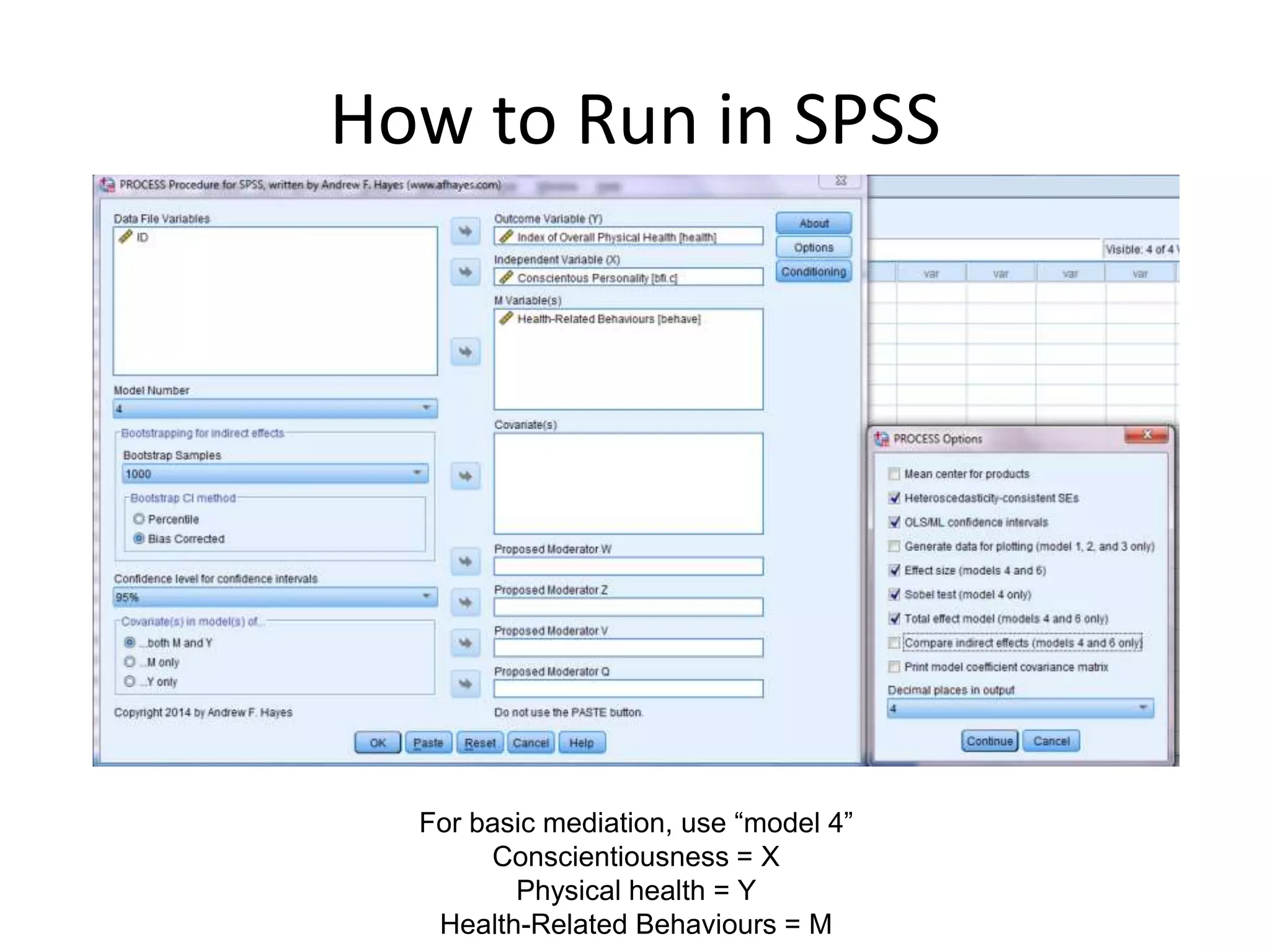
23. How to Run in SPSS
For basic mediation, use “model 4”
Conscientiousness = X
Physical health = Y
Health-Related Behaviours = M

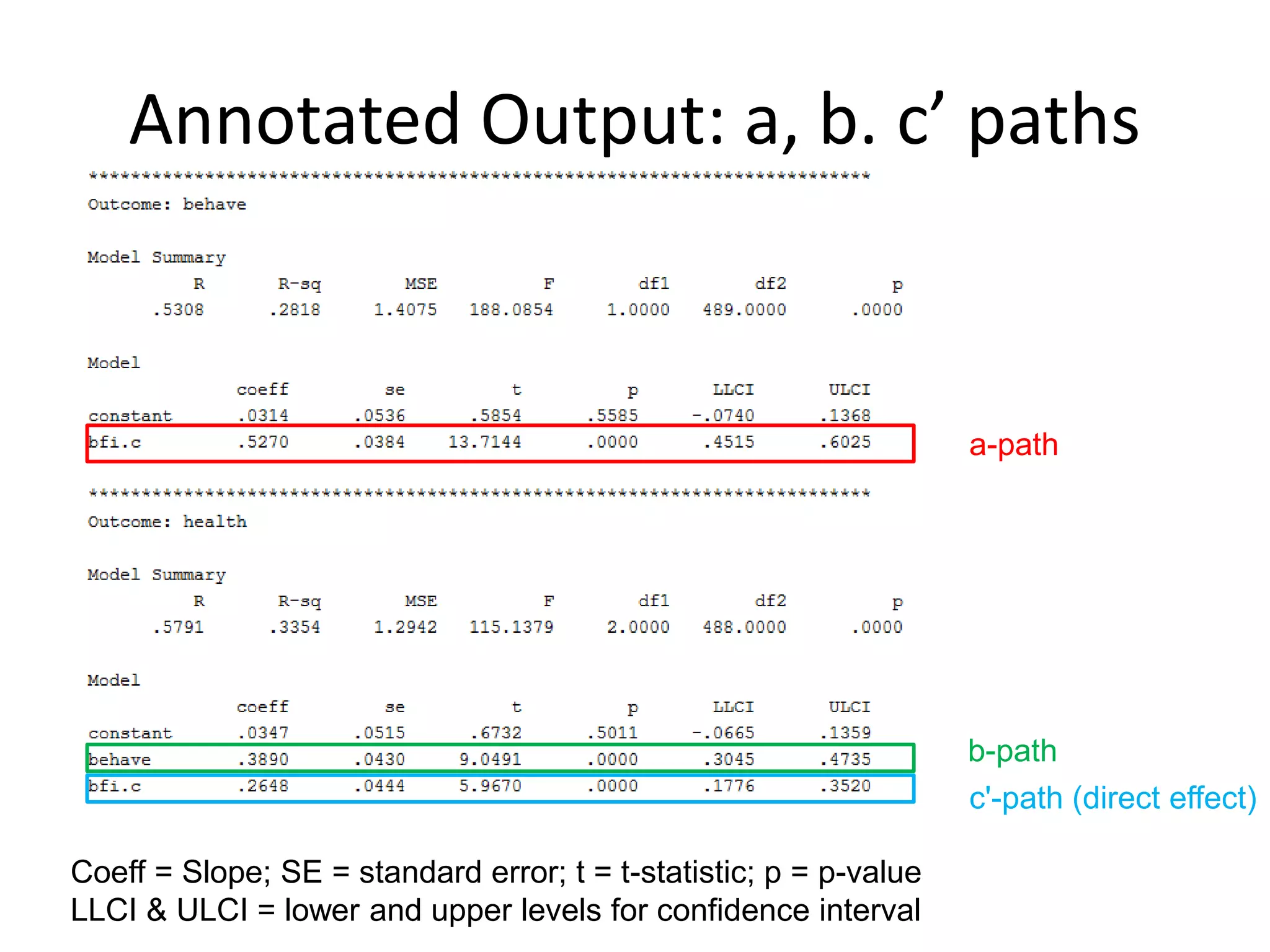
24. Annotated Output: a, b. c’ paths
Coeff = Slope; SE = standard error; t = t-statistic; p = p-value
LLCI & ULCI = lower and upper levels for confidence interval
a-path
b-path
c'-path (direct effect)

25. Annotated Output: c-path
c-path
(total effect)

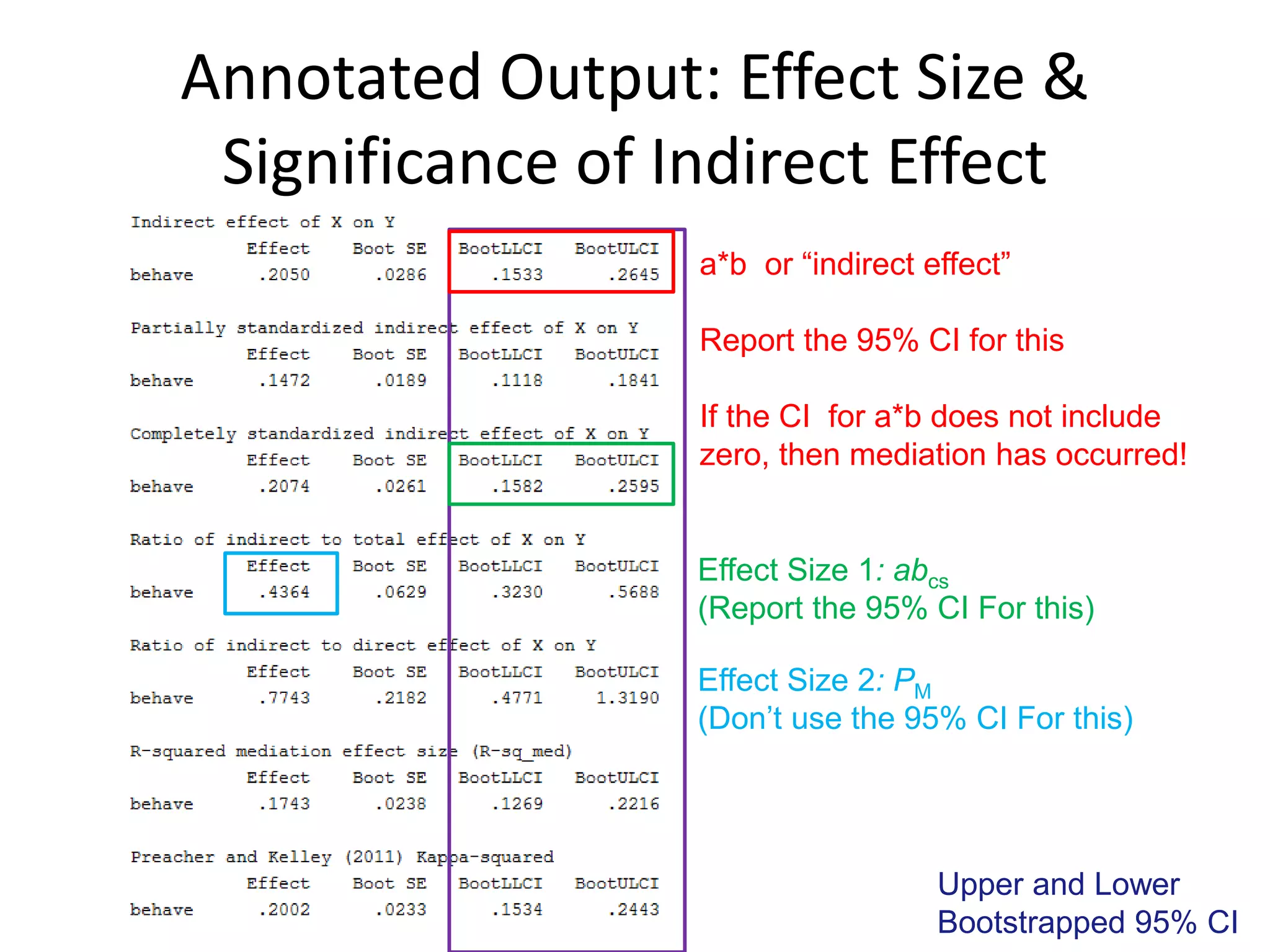
26. Annotated Output: Effect Size &
Significance of Indirect Effect
Effect Size 1: abcs
(Report the 95% CI For this)
Effect Size 2: PM
(Don’t use the 95% CI For this)
Upper and Lower
Bootstrapped 95% CI
a*b or “indirect effect”
Report the 95% CI for this
If the CI for a*b does not include
zero, then mediation has occurred!

27. Reporting Mediation Analysis
There was a significant indirect effect of
conscientiousness on overall physical health through
health-related behaviours, ab = 0.21, BCa CI [0.15,
0.26]. The mediator could account for roughly half of
the total effect, PM = .44.
Conscientious
Personality
Overall Physical
Health
Health-Related
Behaviours0.52*** 0.39***
0.26***
(0.47)***

28. Questions / Contact
Thank you for your time! 
• Email: mackinnon.sean@dal.ca

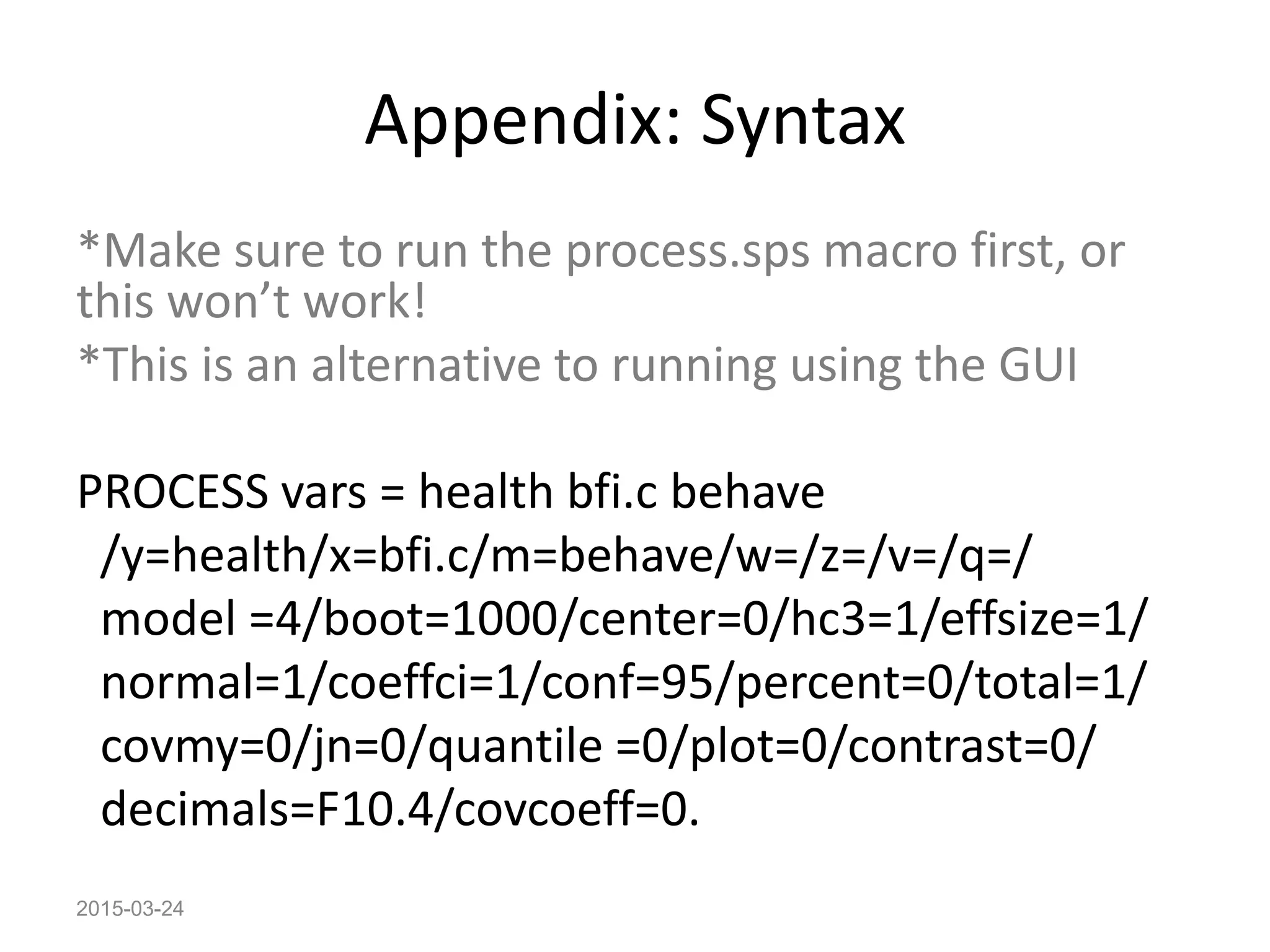
29. Appendix: Syntax
*Make sure to run the process.sps macro first, or
this won’t work!
*This is an alternative to running using the GUI
PROCESS vars = health bfi.c behave
/y=health/x=bfi.c/m=behave/w=/z=/v=/q=/
model =4/boot=1000/center=0/hc3=1/effsize=1/
normal=1/coeffci=1/conf=95/percent=0/total=1/
covmy=0/jn=0/quantile =0/plot=0/contrast=0/
decimals=F10.4/covcoeff=0.
2015-03-24