Assignment DetailsInfluence ProcessesYou have been encourag.docx

Assignment Details:
Influence Processes
You have been encouraged by a colleague to write an article
about "CEOs and presidents" for a management journal. You
have decided to compare the leadership styles of three leaders.
Using the Library, the Internet, and your course materials, write
a 8-10 page report that elaborates on the following:
In your article, provide the following:
· An introduction to the concept of influence processes
· An explanation of the role of influence in contemporary
leadership
· A discussion of the various types of influence processes and
the factors that can affect them
· The methodology used to identify and research the leaders
selected for this report
· An analysis of the influence processes used by the three
leaders. Identify the processes that the leaders and top
management team are using or have used to impact their
organization.
· A discussion of the strengths and weaknesses of the influence
processes used by the three leaders relative to current and future
challenges facing leaders in global organizations.
· A summary of the key attributes of the influence processes
employed by these leaders to effect positive organizational
change or improved performance.
Use the Library or other Web resources to support your
argument. Be sure to cite your sources using APA Style 6th
edition guidelines.
Your report MUST include a reference list. All research should
be cited in the body of the paper. Your report should contain an
abstract, an introduction, and conclusion in addition to the body
of the paper. Please note that if you have a source in your
reference section, you need to cite it in the body of the paper

per APA guidelines and vice-versa.
Deliverable Length: 8-10 pages (body of paper)
©2013 Cengage Learning. All Rights Reserved. May not be
scanned, copied or duplicated, or posted to a publicly accessible
website, in whole or in part.
23
Bivariate Statistical Analysis: Measures of Association
Week 12
*
LEARNING
OUTCOMES
Apply and interpret simple bivariate correlations
Interpret a correlation matrix
Understand simple (bivariate) regression
Understand the least-squares estimation technique
Interpret regression output including the tests of hypotheses tied
to specific parameter coefficients

23-*
Bringing Your Work to Your Home (and Bringing Your Home
to Work)
23-*Work-family conflict (WFC).
Conflict that results when the demands and responsibilities of
one role “spill over” into the other role.Researchers have
examined may work and family characteristics (independent
variables) that can predict WFC (a dependent variable).
The BasicsMeasures of Association
Refers to a number of bivariate statistical techniques used to
measure the strength of a relationship between two variables.
The chi-
two or more less-than interval variables are interrelated.
Correlation analysis is most appropriate for interval or ratio
variables.
Regression can accommodate either less-than interval or
interval independent variables, but the dependent variable must
be continuous.
23–*
*

EXHIBIT 23.1 Bivariate Analysis—Common
Procedures for Testing Association
23–*
*
Correlation coefficient
A statistical measure of the covariation, or association, between
two at-least interval variables.Covariance
Extent to which two variables are associated systematically with
each other.
23–*
Simple Correlation Coefficient (continued)
*

Simple Correlation CoefficientCorrelation coefficient (r)
Ranges from +1 to -1
Perfect positive linear relationship = +1
Perfect negative (inverse) linear relationship = -1
No correlation = 0Correlation coefficient for two variables
(X,Y)
23–*
*
EXHIBIT 23.2 Scatter Diagram to Illustrate Correlation
Patterns
23–*
*
Correlation, Covariance, and CausationWhen two variables
covary, they display concomitant variation.This systematic
covariation does not in and of itself establish causality.e.g.,
Rooster’s crow and the rising of the sun

Rooster does not cause the sun to rise.
23–*
*
Coefficient of DeterminationCoefficient of Determination (R2)
A measure obtained by squaring the correlation coefficient; the
proportion of the total variance of a variable accounted for by
another value of another variable.
Measures that part of the total variance of Y that is accounted
for by knowing the value of X.
23–*
*
Correlation MatrixCorrelation matrix
The standard form for reporting correlation coefficients for
more than two variables.Statistical Significance
The procedure for determining statistical significance is the t-
test of the significance of a correlation coefficient.
23–*

*
EXHIBIT 23.4 Pearson Product-Moment Correlation
Matrix for Salesperson Example
23–*
*
What Makes Attractiveness?
23-*What are the things that make someone attractive?Many
factors are correlated:
Fit
Attractiveness
Weight
Age
Manner of dress (how modern)
Personality (warm versus cold)Results reveal:
Model seems to “fit” the store concept -> attractive.
Overweight -> less attractive
Age -> unrelated to fit or attractiveness

Modernness and perceived coldness -> less attractiveCan help a
retailer determine what employees should look like.
Regression AnalysisSimple (Bivariate) Linear Regression
A measure of linear association that investigates straight-line
relationships between a continuous dependent variable and an
independent variable that is usually continuous, but can be a
categorical dummy variable.The Regression Equation (Y = α +
βX )
Y = the continuous dependent variable
X = the independent variable
α = the Y intercept (regression line intercepts Y axis)
β = the slope of the coefficient (rise over run)
23–*
*
The Regression EquationParameter Estimate Choices
β is indicative of the strength and direction of the relationship
between the independent and dependent variable.
α (Y intercept) is a fixed point that is considered a constant
(how much Y can exist without X)Standardized Regression
Coefficient (β)
Estimated coefficient of the strength of relationship between the

independent and dependent variables.
Expressed on a standardized scale where higher absolute values
indicate stronger relationships (range is from -1 to 1).
23–*
*
The Regression Equation (cont’d)Parameter Estimate Choices
Raw regression estimates (b1)
Raw regression weights have the advantage of retaining the
scale metric—which is also their key disadvantage.
If the purpose of the regression analysis is forecasting, then raw
parameter estimates must be used.
This is another way of saying when the researcher is interested
only in prediction.
Standardized regression estimates (β)
Standardized regression estimates have the advantage of a
constant scale.
Standardized regression estimates should be used when the
researcher is testing explanatory hypotheses.
23–*
*

EXHIBIT 23.7 The Best-Fit Line or Knocking Out the
Pins
23–*
*
OLS
Guarantees that the resulting straight line will produce the least
possible total error in using X to predict Y.
Generates a straight line that minimizes the sum of squared
deviations of the actual values from this predicted regression
line.
No straight line can completely represent every dot in the
scatter diagram.
There will be a discrepancy between most of the actual scores
(each dot) and the predicted score .
Uses the criterion of attempting to make the least amount of
total error in prediction of Y from X.
23–*
Ordinary Least-Squares (OLS) Method of Regression Analysis
*

23–*
Ordinary Least-Squares Method of Regression Analysis (OLS)
(cont’d)
*
The equation means that the predicted value for any value of X
(Xi) is determined as a function of the estimated slope
coefficient, plus the estimated intercept coefficient + some
error.
23–*
(cont’d)
*
23–*
(cont’d)

*
Statistical Significance Of Regression ModelF-test (regression)
Determines whether more variability is explained by the
regression or unexplained by the regression.
23–*
(cont’d)
*
R2
The proportion of variance in Y that is explained by X (or vice
versa)
A measure obtained by squaring the correlation coefficient; that
proportion of the total variance of a variable that is accounted
for by knowing the value of another variable.
23–*
(cont’d)
*

EXHIBIT 23.8 Simple Regression Results for Building
Permit Example
23–*
*
EXHIBIT 23.9 OLS Regression Line
23–*
*
Size and Weight

23-*The fight to get thin is a multibillion dollar business.H1:
Perceptions that a female model is overweight are related
negatively to perceptions of attractiveness.Can be tested with
simple regression.The results support the hypothesis.
Simple Regression and Hypothesis TestingThe explanatory
power of regression lies in hypothesis testing. Regression is
often used to test relational hypotheses.
The outcome of the hypothesis test involves two conditions that
must both be satisfied:
The regression weight must be in the hypothesized direction.
Positive relationships require a positive coefficient and negative
relationships require a negative coefficient.
The t-test associated with the regression weight must be
significant.
23–*
(
)
(
)
(
)
(
)
å
å
å
=
=
=
-

-
-
-
=
=
n
i
n
i
n
i
i
i
yx
xy
Y
Yi
X
Xi
Y
Y
X
X
r
r
1
1
2
2
1
Variance
Total
variance
Explained
2

=
R
875
.
0
40
.
882
,
3
49
.
398
,
3
2
=
=
R
23
Bivariate Statistical Analysis: Measures of Association
Week 12
*

LEARNING
OUTCOMES
Apply and interpret simple bivariate correlations
Interpret a correlation matrix
Understand simple (bivariate) regression
Understand the least-squares estimation technique
Interpret regression output including the tests of hypotheses tied
to specific parameter coefficients
23-*
Bringing Your Work to Your Home (and Bringing Your Home
to Work)
23-*Work-family conflict (WFC).
Conflict that results when the demands and responsibilities of
one role “spill over” into the other role.Researchers have
examined may work and family characteristics (independent
variables) that can predict WFC (a dependent variable).
The BasicsMeasures of Association

Refers to a number of bivariate statistical techniques used to
measure the strength of a relationship between two variables.
The chi-
two or more less-than interval variables are interrelated.
Correlation analysis is most appropriate for interval or ratio
variables.
Regression can accommodate either less-than interval or
interval independent variables, but the dependent variable must
be continuous.
23–*
*
EXHIBIT 23.1 Bivariate Analysis—Common
Procedures for Testing Association
23–*
*
Correlation coefficient
A statistical measure of the covariation, or association, between
two at-least interval variables.Covariance

Extent to which two variables are associated systematically with
each other.
23–*
Simple Correlation Coefficient (continued)
*
Simple Correlation CoefficientCorrelation coefficient (r)
Ranges from +1 to -1
Perfect positive linear relationship = +1
Perfect negative (inverse) linear relationship = -1
No correlation = 0Correlation coefficient for two variables
(X,Y)
23–*
*
EXHIBIT 23.2 Scatter Diagram to Illustrate Correlation
Patterns

23–*
*
Correlation, Covariance, and CausationWhen two variables
covary, they display concomitant variation.This systematic
covariation does not in and of itself establish causality.e.g.,
Rooster’s crow and the rising of the sun
Rooster does not cause the sun to rise.
23–*
*
Coefficient of DeterminationCoefficient of Determination (R2)
A measure obtained by squaring the correlation coefficient; the
proportion of the total variance of a variable accounted for by
another value of another variable.
Measures that part of the total variance of Y that is accounted
for by knowing the value of X.
23–*

*
Correlation MatrixCorrelation matrix
The standard form for reporting correlation coefficients for
more than two variables.Statistical Significance
The procedure for determining statistical significance is the t-
test of the significance of a correlation coefficient.
23–*
*
EXHIBIT 23.4 Pearson Product-Moment Correlation
Matrix for Salesperson Example
23–*
*

What Makes Attractiveness?
23-*What are the things that make someone attractive?Many
factors are correlated:
Fit
Attractiveness
Weight
Age
Manner of dress (how modern)
Personality (warm versus cold)Results reveal:
Model seems to “fit” the store concept -> attractive.
Overweight -> less attractive
Age -> unrelated to fit or attractiveness
Modernness and perceived coldness -> less attractiveCan help a
retailer determine what employees should look like.
Regression AnalysisSimple (Bivariate) Linear Regression
A measure of linear association that investigates straight-line
relationships between a continuous dependent variable and an
independent variable that is usually continuous, but can be a
categorical dummy variable.The Regression Equation (Y = α +
βX )
Y = the continuous dependent variable
X = the independent variable
α = the Y intercept (regression line intercepts Y axis)
β = the slope of the coefficient (rise over run)
23–*

*
The Regression EquationParameter Estimate Choices
β is indicative of the strength and direction of the relationship
between the independent and dependent variable.
α (Y intercept) is a fixed point that is considered a constant
(how much Y can exist without X)Standardized Regression
Coefficient (β)
Estimated coefficient of the strength of relationship between the
independent and dependent variables.
Expressed on a standardized scale where higher absolute values
indicate stronger relationships (range is from -1 to 1).
23–*
*
The Regression Equation (cont’d)Parameter Estimate Choices
Raw regression estimates (b1)
Raw regression weights have the advantage of retaining the
scale metric—which is also their key disadvantage.
If the purpose of the regression analysis is forecasting, then raw
parameter estimates must be used.
This is another way of saying when the researcher is interested

only in prediction.
Standardized regression estimates (β)
Standardized regression estimates have the advantage of a
constant scale.
Standardized regression estimates should be used when the
researcher is testing explanatory hypotheses.
23–*
*
EXHIBIT 23.7 The Best-Fit Line or Knocking Out the
Pins
23–*
*
OLS
Guarantees that the resulting straight line will produce the least
possible total error in using X to predict Y.
Generates a straight line that minimizes the sum of squared
deviations of the actual values from this predicted regression
line.

No straight line can completely represent every dot in the
scatter diagram.
There will be a discrepancy between most of the actual scores
(each dot) and the predicted score .
Uses the criterion of attempting to make the least amount of
total error in prediction of Y from X.
23–*
Ordinary Least-Squares (OLS) Method of Regression Analysis
*
23–*
(cont’d)
*
The equation means that the predicted value for any value of X
(Xi) is determined as a function of the estimated slope
coefficient, plus the estimated intercept coefficient + some
error.
23–*

(cont’d)
*
23–*
(cont’d)
*
Statistical Significance Of Regression ModelF-test (regression)
Determines whether more variability is explained by the
regression or unexplained by the regression.
23–*
(cont’d)
*

R2
The proportion of variance in Y that is explained by X (or vice
versa)
A measure obtained by squaring the correlation coefficient; that
proportion of the total variance of a variable that is accounted
for by knowing the value of another variable.
23–*
(cont’d)
*
EXHIBIT 23.8 Simple Regression Results for Building
Permit Example
23–*
*

EXHIBIT 23.9 OLS Regression Line
23–*
*
Size and Weight
23-*The fight to get thin is a multibillion dollar business.H1:
Perceptions that a female model is overweight are related
negatively to perceptions of attractiveness.Can be tested with
simple regression.The results support the hypothesis.
Simple Regression and Hypothesis TestingThe explanatory
power of regression lies in hypothesis testing. Regression is
often used to test relational hypotheses.
The outcome of the hypothesis test involves two conditions that
must both be satisfied:
The regression weight must be in the hypothesized direction.
Positive relationships require a positive coefficient and negative
relationships require a negative coefficient.
The t-test associated with the regression weight must be
significant.
23–*

(
)
(
)
(
)
(
)
å
å
å
=
=
=
-
-
-
-
=
=
n
i
n
i
n
i
i
i
yx
xy
Y
Yi
X
Xi
Y
Y

X
X
r
r
1
1
2
2
1
Variance
Total
variance
Explained
2
=
R
875
.
0
40
.
882
,
3
49
.
398
,
3
2
=
=
R

CorrRegr-SPSS.docx
Correlation and Regression Analysis: SPSS
Bivariate Analysis: Cyberloafing Predicted from Personality
and Age
These days many employees, during work hours, spend time on
the Internet doing personal
things, things not related to their work. This is called
“cyberloafing.” Research at ECU, by Mike
Sage, graduate student in Industrial/Organizational Psychology,
has related the frequency of
cyberloafing to personality and age. Personality was measured
with a Big Five instrument.
Cyberloafing was measured with an instrument designed for this
research. Age is in years. The
cyberloafing instrument consisted of 23 questions about
cyberloafing behaviors, such as “shop online
for personal goods,” “send non-work-related e-mail,” and “use
Facebook.” For each item,
respondents were asked how often they engage in the specified
activity during work hours for
personal reasons. The response options were “Never,” “Rarely
(about once a month),” “Sometimes
(at least once a week),” and “Frequently (at least once a day).”
Higher scores indicate greater
frequency of cyberloafing.
For this exercise, the only Big Five
personality factor we shall use is that for

Conscientiousness. Bring the data,
Cyberloaf_Consc_Age.sav, into SPSS. Click
Analyze, Descriptive Statistics, Frequencies.
Scoot all three variables into the pane on the
right. Uncheck “Display frequency tables.
Click on “Statistics” and select the statistics shown below.
Continue. Click on “Charts” and
select the charts shown below. Continue. OK.
Copyright 2016, Karl L. Wuensch - All rights reserved.
http://www.ecu.edu/cs-cas/psyc/IO-Home.cfm
https://www.google.com/search?rlz=1C2GGGE_enUS414US459
&num=50&safe=off&site=&source=hp&q=big+five+personality
&oq=big+five+personality&gs_l=hp.3..0l10.97045.104685.0.10
5496.21.12.0.9.9.0.232.1521.1j10j1.12.0.msedr...0...1c.1.64.hp..
1.20.1383.0.jmw-YtTw8h4
http://core.ecu.edu/psyc/wuenschk/SPSS/Cyberloaf_Consc_Age.
sav
2
The output will show that age is positively skewed, but not
quite badly enough to require us to
transform it to pull in that upper tail. Click Analyze, Correlate,
Bivariate. Move all three variables into
the Variables box. Ask for Pearson and Spearman coefficients,

two-tailed, flagging significant
coefficients. Click OK. Look at the output. With both Pearson
and Spearman, the correlations
between cyberloafing and both age and Conscientiousness are
negative, significant, and of
considerable magnitude. The correlation between age and
Conscientiousness is small and not
significant.
Click Analyze, Regression, Linear. Scoot the Cyberloafing
variable into the Dependent box
and Conscientiousness into the Independent(s) box.
3
Click Statistics. Select the statistics shown below. Continue.
Click Plots. Select the plot
shown below. Continue, OK.
Look at the output. The “Model Summary” table reports the
same value for Pearson r obtained
with the correlation analysis, of course. The r
2
shows that our linear model explains 32% of the

variance in cyberloafing. The adjusted R
2
, also known as the “shrunken R
2
,” is a relatively unbiased
2
. For a bivariate regression it is computed as:
)2(
)1)(1(
1
2
2
n
nr
r
shrunken .
Model Summary
b

Model R R Square Adjusted R
Square
Std. Error of the
Estimate
1 .563
a
.317 .303 7.677
a. Predictors: (Constant), Conscientiousness
b. Dependent Variable: Cyberloafing
The regression coefficients are shown in a table labeled
“Coefficients.”
Coefficients
a
Model Unstandardized Coefficients Standardized
Coefficients
t Sig.
B Std. Error Beta
1
(Constant) 57.039 7.288

7.826 .000
Conscientiousness -.864 .181 -.563 -4.768 .000
4
The general form of a bivariate regression equation is “Y = a +
bX.” SPSS calls the Y
variable the “dependent” variable and the X variable the
“independent variable.” I think this notation
is misleading, since regression analysis is frequently used with
data collected by nonexperimental
means, so there really are not “independent” and “dependent”
variable.
In “Y = a + bX,” a is the intercept (the predicted value for Y
when X = 0) and b is the slope (the
number of points that Y changes, on average, for each one point
change in X. SPSS calls a the
“constant.” The slope is given in the “B” column to the right of
the name of the X variable. SPSS also
regression is identical to the Pearson r.
For the data at hand, the regression equation is “cyberloafing =
57.039 - .864 consciousness.”

The residuals statistics show that there no cases with a
standardized residual beyond three
standard deviations from zero. If there were, they would be
cases where the predicted value was
very far from the actual value and we would want to investigate
such cases. The histogram shows
that the residuals are approximately normally distributed, which
is assumed when we use t or F to get
a p value or a confidence interval.
Let’s now create a scatterplot. Click Graphs, Legacy Dialogs,
Scatter/Dot, Simple Scatter,
Define. Scoot Cyberloafing into the Y axis box and
Conscientiousness into the X axis box. Click OK.
Go to the Output window and double click on the chart to open
the chart editor. Click
Elements, Fit Line at Total, Fit Method = Linear, Close.
5
You can also ask SPSS to
draw confidence bands on the plot,
for predicting the mean Y given X,
or individual Y given X, or both (to
get both, you have to apply the one,
close the editor, open the editor
again, apply the other).

You can also edit the shape, density, and color of the markers
and the lines. While in the
Chart Editor, you can Edit, Copy Chart and then paste the chart
into Word. You can even ask SPSS
6
to put in a quadratic (Y = a +b1X + b2X
2
+ error) or cubic (Y = a +b1X + b2X
2
+b3X
3
+ error)
regression line.
With a more recent version of SPSS, the plot with the
regression line included the regression
equation superimposed onto the line. I did not like that, and
spent too long trying to make it go away,
without success, but with much cussing. Then one of brilliant
graduate students, Jennifer Donelan,
told me how to make it go away. See the new window below.
If you uncheck the “Attach label to line”
box, that pesky equation goes away.

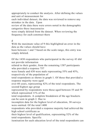
Vassar. Enter the value of r and
sample size and click “Calculate.”
http://vassarstats.net/rho.html
7
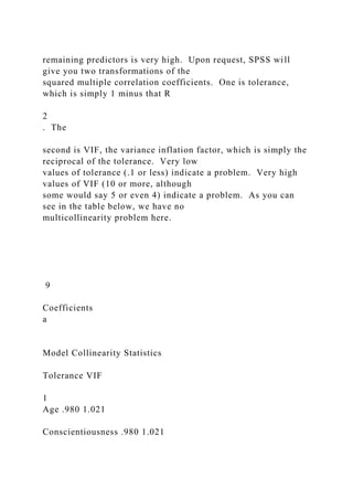
Presenting the Results of a Correlation/Regression Analysis.
Employees’ frequency of
cyberloafing (CL) was found to be significantly, negatively
correlated with their Conscientiousness
(CO), CL = 57.039 - .864 CO, r(N = 51) = -.563, p < .001, 95%
CI [-.725, -.341].
Trivariate Analysis: Age as a Second Predictor
Click Analyze, Regression, Linear. Scoot the Cyberloafing
variable into the Dependent box
and both Conscientiousness and Age into the Independents box.
Click Statistics and check Part and
Partial Correlations, Casewise Diagnostics, and Collinearity
Diagnostics (Estimates and Model Fit
should already be checked). Click Continue. Click Plots.
Scoot *ZRESID into the Y box and
*ZPRED into the X box. Check the Histogram box and then
click Continue. Click Continue, OK.
When you look at the output for this multiple regression, you
see that the two predictor model

does do significantly better than chance at predicting
cyberloafing, F(2, 48) = 20.91, p < .001. The F
in the ANOVA table tests the null hypothesis that the multiple
correlation coefficient, R, is zero in the
population. If that null hypothesis were true, then using the
regression equation would be no better
than just using the mean for cyberloafing as the predicted
cyberloafing score for every person.
Clearly we can predict cyberloafing significantly better with the
regression equation rather than
without it, but do we really need the age variable in the model?
Is this model significantly better than
the model that had only Conscientiousness as a predictor? To
answer that question, we need to look
at the "Coefficients," which give us measures of the partial
effect of each predictor, above and beyond
the effect of the other predictor(s).
8
The Regression Coefficients
The regression equation gives us two unstandardized slopes,
both of which are partial
statistics. The amount by which cyberloafing changes for each
one point increase in
Conscientiousness, above and beyond any change associated
with age, is -.779, and the amount by
which cyberloafing changes for each one point increase in age,
above and beyond any change
associated with Conscientiousness, is -.276. The intercept,
64.07, is just a reference point, the
predicted cyberloafing score for a person whose

Conscientiousness and age are both zero (which are
not even possible values). The "Standardized Coefficients"
standardized units -- that is, how many standard deviations does
cyberloafing change for each one
standard deviation increase in the predictor, above and beyond
the effect of the other predictor(s).
The regression equation represents a plane in three dimensional
space (the three dimensions
being cyberloafing, Conscientiousness, and age). If we plotted
our data in three dimensional space,
that plane would minimize the sum of squared deviations
between the data and the plane. If we had
a 3
rd
predictor variable, then we would have four dimensions, each
perpendicular to each other
dimension, and we would be out in hyperspace.
Tests of Significance
The t testing the null hypothesis that the intercept is zero is of
no interest, but those testing the
partial slopes are. Conscientiousness does make a significant,
unique, contribution towards
predicting AR, t(48) = 4.759, p < .001. Likewise, age also
makes a significant, unique, contribution,
t(48) = 3.653, p = .001 Please note that the values for the
partial coefficients that you get in a
multiple regression are highly dependent on the context
provided by the other variables in a model. If
you get a small partial coefficient, that could mean that the

predictor is not well associated with the
dependent variable, or it could be due to the predictor just being
highly redundant with one or more of
the other variables in the model. Imagine that we were foolish
enough to include, as a third predictor
in our model, students’ score on the Conscientiousness and age
variables added together. Assume
that we made just a few minor errors when computing this sum.
In this case, each of the predictors
would be highly redundant with the other predictors, and all
would have partial coefficients close to
zero. Why did I specify that we made a few minor errors when
computing the sum? Well, if we didn’t,
then there would be total redundancy (at least one of the
predictor variables being a perfect linear
combination of the other predictor variables), which causes the
intercorrelation matrix among the
predictors to be singular. Singular intercorrelation matrices
cannot be inverted, and inversion of that
matrix is necessary to complete the multiple regression analysis.
In other words, the computer
program would just crash. When predictor variables are highly
(but not perfectly) correlated with one
another, the program may warn you of multicollinearity. This
problem is associated with a lack of
stability of the regression coefficients. In this case, were you
randomly to obtain another sample from
the same population and repeat the analysis, there is a very
good chance that the results (the
estimated regression coefficients) would be very different.
Multicollinearity
Multicollinearity is a problem when for any predictor the R
2
between that predictor and the

remaining predictors is very high. Upon request, SPSS will
give you two transformations of the
squared multiple correlation coefficients. One is tolerance,
which is simply 1 minus that R
2
. The
second is VIF, the variance inflation factor, which is simply the
reciprocal of the tolerance. Very low
values of tolerance (.1 or less) indicate a problem. Very high
values of VIF (10 or more, although
some would say 5 or even 4) indicate a problem. As you can
see in the table below, we have no
multicollinearity problem here.
9
Coefficients
a
Model Collinearity Statistics
Tolerance VIF
1
Age .980 1.021
Conscientiousness .980 1.021

Partial and Semipartial Correlation Coefficients
I am going to use a Venn diagram to help explain what squared
partial and semipartial
correlation coefficients are.. Look at the ballantine below.
The top circle represents variance in cyberloafing, the right
circle that in age, the left circle that in
Conscientiousness. The overlap between circle Age and
Cyberloaf, area A + B, represents the r
2
between cyberloafing and age. Area B + C represents the r
2
between cyberloafing and
Conscientiousness. Area A + B + C + D represents all the
variance in cyberloafing, and we
standardize it to 1. Area A + B + C represents the variance in
cyberloafing explained by our best
weighted linear combination of age and Conscientiousness,
46.6% (R
2
). The proportion of all of the
variance in cyberloafing which is explained by age but not by
Conscientiousness is equal to:
A
A

DCBA
A
.
Area A represents the squared semipartial correlation for age
(.149). Area C represents the
squared semipartial correlation for Conscientiousness (.252).
SPSS gives you the unsquared
semipartial correlation coefficients, but calls them "part
correlations."
Although I generally prefer semipartial correlation coefficients,
some persons report the partial
correlation coefficients, which are provided by SPSS. The
partial correlation coefficient will always
be at least as large as the semipartial, and almost always larger.
To treat it as a proportion, we
obtain the squared partial correlation coefficient. In our Venn
diagram, the squared partial
correlation coefficient for Conscientiousness is represented by
the proportion
DC
C
. That is, of the
variance in cyberloafing that is not explained by age, what
proportion is explained by
Conscientiousness? Or, put another way, if we already had age

in our prediction model, by what
proportion could we reduce the error variance if we added
Conscientiousness to the model? If you
consider that (C + D) is between 0 and 1, you should understand
why the partial coefficient will be
larger than the semipartial.
If we take age back out of the model, the r
2
drops to .317. That drop, .466 - .317 = .149, is the
squared semipartial correlation coefficient for age. In other
words, we can think of the squared
semipartial correlation coefficient as the amount by which the R
2
drops if we delete a predictor from
the model.
http://www.amstat.org/publications/jse/v10n1/kennedy.html
10
If we refer back to our Venn diagram, the R
2
is represented by the area A+B+C, and the
redundancy between misanthropy and idealism by area B. The
redundant area is counted (once) in
the multiple R
2
, but not in the partial statistics.

Checking the Residuals
For each subject, the residual is the subject’s actual Y score
minus the Y score as predicted
from the regression solution. When we use t or F to test
hypotheses about regression parameters or
to construct confidence intervals, we assume that, in the
population, those residuals are normally
distributed and constant in variance.
The histogram shows the marginal distribution of the residuals.
We have assumed that this is
normal.
The plot of the standardized residuals (standardized difference
between actual cyberloafing
score and that predicted from the model) versus standardized
predicted values allows you to evaluate
the normality and homescedasticity assumptions made when
testing the significance of the model
and its parameters. Open the chart in the editor and click
Options, Y-axis reference line to draw a
horizontal line at residual = 0. If the normality assumption has
been met, then a vertical column of
residuals at any point on that line will be normally distributed.
In that case, the density of the plotted
symbols will be greatest near that line, and drop quickly away
from the line, and will be symmetrically
distributed on the two sides (upper versus lower) of the line. If
the homoscedasticity assumption
has been met, then the spread of the dots, in the vertical
dimension, will be the same at any one point
on that line as it is at any other point on that line. Thus, a
residuals plot can be used, by the trained
eye, to detect violations of the assumptions of the regression
analysis. The trained eye can also

detect, from the residual plot, patterns that suggest that the
relationship between predictor and
criterion is not linear, but rather curvilinear.
Residuals can also be used to identify any cases with large
residuals – that is, cases where
the actual Y differs greatly from the predicted Y. Such cases
are suspicious and should be
investigated. They may represent for which the data were
incorrectly entered into the data file or for
which there was some problem during data collection. They
may represent cases that are not
properly considered part of the population to which we wish to
generalize our results. One should
investigate cases where the standardized residual has an
absolute value greater than 3 (some would
say 2).
11
Importance of Looking at a Scatterplot Before You Analyze
Your Data
It is very important to look at a plot of your data prior to
conducting a linear
correlation/regression analysis. Close the
Cyberloaf_Consc_Age.sav file and bring Corr_Regr.sav
into SPSS. From the Data Editor, click Data, Split File,
Compare Groups, and scoot Set into the
"Organize output by groups" box. Click OK.

Next, click Analyze, Regression, Linear. Scoot Y into the
Dependent box and X into the
Independent(s) box. Click Stat and ask for Descriptives
(Estimates and Model Fit should already be
selected). Click Continue, OK.
Next, click Graphs, Scatter, Simple. Identify Y as the Y
variable and X as the X variable. Click
OK.
Look at the output. For each of the data sets, the mean on X is
9, the mean on Y is 7.5, the
standard deviation for X is 3.32, the standard deviation for Y is
2.03, the r is .816, and the regression
equation is Y = 3 + .5X – but now look at the plots. In Set A,
we have a plot that looks about like what
we would expect for a moderate to large positive correlation. In
set B we see that the relationship is
really curvilinear, and that the data could be fit much better
with a curved line (a polynomial function,
quadratic, would fit them well). In Set C we see that, with the
exception of one outlier, the relationship
is nearly perfect linear. In set D we see that the relationship
would be zero if we eliminated the one
extreme outlier -- with no variance in X, there can be no
covariance with Y.
Moderation Analysis
Sometimes a third variable moderates (alters) the relationship
between two (or more) variables
of interest. You are about to learn how to conduct a simple
moderation analysis.

One day as I sat in the living room, watching the news on TV,
there was a story about some
demonstration by animal rights activists. I found myself
agreeing with them to a greater extent than I
normally do. While pondering why I found their position more
appealing than usual that evening, I
noted that I was also in a rather misanthropic mood that day.
That suggested to me that there might
be an association between misanthropy and support for animal
rights. When evaluating the ethical
status of an action that does some harm to a nonhuman animal, I
generally do a cost/benefit analysis,
weighing the benefit to humankind against the cost of harm
done to the nonhuman. When doing such
an analysis, if one does not think much of humankind (is
misanthropic), e is unlikely to be able to
justify harming nonhumans. To the extent that one does not
like humans, one will not be likely to
think that benefits to humans can justify doing harm to
nonhumans. I decided to investigate the
relationship between misanthropy and support of animal rights.
Mike Poteat and I developed an animal rights questionnaire,
and I developed a few questions
designed to measure misanthropy. One of our graduate
students, Kevin Jenkins, collected the data
http://core.ecu.edu/psyc/wuenschk/SPSS/Corr_Regr.sav
12
we shall analyze here. His respondents were students at ECU. I
used reliability and factor
analysis to evaluate the scales (I threw a few items out). All of
the items were Likert-type items, on a

5-point scale. For each scale, we computed each respondent's
mean on the items included in that
scale. The scale ran from 1 (strongly disagree) to 5 (strongly
agree). On the Animal Rights scale
(AR), high scores represent support of animal rights positions
(such as not eating meat, not wearing
leather, not doing research on animals, etc.). On the
Misanthropy scale (MISANTH), high scores
represent high misanthropy (such as agreeing with the statement
that humans are basically wicked).
The idealist is one who believes that morally correct behavior
always leads only to desirable
consequences; an action that leads to any bad consequences is a
morally wrong action. Thus, one
would expect the idealist not to engage in cost/benefit analysis
of the morality of an action -- any bad
consequences cannot be cancelled out by associated good
consequences. Thus, there should not
be any relationship between misanthropy and attitude about
animals in idealists, but there should be
such a relationship in nonidealists (who do engage in such
cost/benefit analysis, and who may, if they
are misanthropic, discount the benefit to humans).
Accordingly, a proper test of my hypothesis would be one that
compared the relationship
between misanthropy and attitude about animals for idealists
versus for nonidealists. Although I did a
more sophisticated analysis than is presented here (a "Potthoff
analysis," which I cover in my
advanced courses), the analysis presented here does address the
question I posed. Based on a
scores on the measure of idealism, each participant was
classified as being either an idealist or not
an idealist. Now all we need to do is look at the relationship

between misanthropy and idealism
separately for idealists and for nonidealists.
Bring into SPSS the data file Poffhoff.sav. From the Data
Editor, click Data, Split File,
Organize Output by Groups. Scoot the Idealism variable into
the "Groups based on" box. Click OK.
Click Analyze, Regression, Linear. Scoot AR into the
Dependent box, Misanth into the
Independent(s) box. Click Statistics. Check Descriptives
(Estimates and Model Fit should already be
checked). Click Continue, OK.
Make some scatter plots too, with the regression line drawn in.
Click Graphs, Legacy
Dialogues, Scatter/Dot, Simple Scatter, Define. Scoot AR into
the Y axis box and Misanth into the X
axis box. Click OK. Go to the Output window and double click
on each chart to open the chart editor.
Click Elements, Fit Line at Total, Fit Method = Linear, Close.
The output for the nonidealists shows that the relationship
between attitude about animals and
misanthropy is significant ( p < .001) and of nontrivial
magnitude ( r = .364, n = 91). The plot shows a
nice positive slope for the regression line. With nonidealists,
misanthropy does produce a discounting
of the value of using animals for human benefit, and,
accordingly, stronger support for animal rights.
On the other hand, with the idealists, who do not do cost/benefit
analysis, there is absolutely no
relationship between misanthropy and attitude towards animals.
The correlation is trivial ( r = .020, n
= 63) and nonsignificant ( p = .87), and the plot shows the
regression line to be flat.

You can find a paper based on these data at:
http://core.ecu.edu/psyc/wuenschk/Animals/ABS99-ppr.htm
Group Differences in Unstandardized Slopes and in Correlation
Coefficients
Please remember that the relationship between X and Y could
differ with respect to the slope
for predicting Y from X, but not with respect to the Pearson r,
or vice versa The Pearson r really
measures how little scatter there is around the regression line
(error in prediction), not how steep the
regression line is.
http://core.ecu.edu/psyc/wuenschk/SPSS/POTTHOFF.sav
http://core.ecu.edu/psyc/wuenschk/Animals/ABS99-ppr.htm
13
On the left, we can see that the slope is the same for the
relationship plotted with blue o’s and
that plotted with red x’s, but there is more error in prediction (a
smaller Pearson r ) with the blue o’s.
For the blue data, the effect of extraneous variables on the
predicted variable is greater than it is with
the red data.
On the right, we can see that the slope is clearly higher with the

red x’s than with the blue o’s,
but the Pearson r is about the same for both sets of data. We
can predict equally well in both groups,
but the Y variable increases much more rapidly with the X
variable in the red group than in the blue.
Placing a Confidence Interval on Multiple R or R
2
Please see my document Putting Confidence Intervals on R
2
or R.
Presenting the Results of a Multiple Linear
Correlation/Regression Analysis
Please read the article at
http://jolt.merlot.org/vol5no2/wuensch_0609.pdf and pay
special
attention to how the results of the multiple regression analyses
were presented, including Tables 3
and 4. This is the style I would expect you to use when
presenting the results of a multiple regression
were such an analysis to be on the an assignment or
examination.
Annotated Output for This Lesson
Return to my SPSS Lessons page
More Lessons on Multiple Regression
Multiple Regression With SAS

Producing and Interpreting Residuals Plots in SPSS
Copyright 2019, Karl L. Wuensch - All rights reserved.
http://core.ecu.edu/psyc/wuenschk/docs30/CI-R2.docx
http://jolt.merlot.org/vol5no2/wuensch_0609.pdf
http://core.ecu.edu/psyc/wuenschk/SPSS/Corr-Regr-SPSS-
Output.pdf
http://core.ecu.edu/psyc/wuenschk/SPSS/SPSS-Lessons.htm
http://core.ecu.edu/psyc/wuenschk/StatsLessons.htm#MultReg
http://core.ecu.edu/psyc/wuenschk/SAS/SAS-
MV.htm#MultipleRegression
http://core.ecu.edu/psyc/wuenschk/SPSS/Residual-Plots-
SPSS.doc
Assessment 3
This report has been developed at the request of senior
management to understand the
relationship between customer participation and service firm
performance to help improve
business practices.
Preliminary Analysis
The sample for this study is drawn from data collected from the
data service industry. In total
there were 1430 questionnaires distributed.
Prior to conducting any analysis, the data set was cleaned to
ensure the data could be used

appropriately to conduct the analysis. After defining the values
and unit of measurement for
each individual dataset, the data was reviewed to remove any
mistakes in the data. Upon
review of the data there were errors noted in the demographic
categories these inaccuracies
were simply deleted from the dataset. When reviewing the
frequency for each construct there
d
With the maximum value of 9 this highlighted an error in the
data as the values should have
been between 1 and 7 based on the scale range, this entry was
simply deleted.
Of the 1430 respondents who participated in the survey 43 did
not provide information
related to their gender, from the remaining 1387 participants
who provided a response 757
were female and 630 were male representing 55% and 45%,
respectively of the population of
total respondents as shown in graph 1. Of those that provided a
response majority were aged
over 60 years, representing 42% of the total respondents. The
second highest age group
represented by respondents were those aged between 55 and 59
which represented 11% of the
total respondents. A complete breakdown of the age brackets
can be seen in graph 2. Due to
incomplete data for the highest level of education, 30 surveys
were omitted. Of the total 1400
respondents who provided a response majority had achieved the
high school certificate as
their highest level of qualification, representing 52% of the
total respondents. Specific
itemisation for each education level of the total respondents can

be seen in table 1 and graph
3. Of the 1390 who provided a response to the frequency for use
of service brand majority
indicated they used the brand on a weekly basis representing
38% of total respondents.
The survey captured information relating to customer perception
of employee customer
orientation, customer participation, customer satisfaction,
customer willingness to pay and
customer perception of brand image. The constructs were
measured using a 7 point Likert
scale which is the most common scale used for data collection.
The results of kortosis and skewness show that some items are
normally distributed. These
items are customer participation (CCP1-CCP5), customer
willingness to pay (WP1-WP2) and
customer perception of brand image (B11-B17) as the kurtosis
indices fitted between 3 and
skewness indices fitted between 1 we can conclude these items
have normal distributions.
Items including customer perception (EC01-EC06) and customer
satisfaction (CS1-CS2) are
not normally distributed although the kurtosis indices fitted
between 3 the skewness indices
do not fit between 1. The complete results of kortisis and
skewness testing as well as the
mean and standard deviation for each construct can be seen
below in table 2, descriptive
statistics.
The factor loading for each construct was measured as part of
the preliminary analysis of
data. As a well accepted rule, the factor loading for all items
should be over 0.5 and no cross

loading should be detected. As shown in table 3, preliminary
analysis all of the factor loading
scores for all constructs are greater than 0.5, which shows the
measures used in this study
have acceptable convergent validity.
The composite reliability for all constructs was calculated, as
detailed in table 3, preliminary
analysis. The results show that composite reliability scores for
customer perception of
employee customer orientation, customer participation and
customer perception of brand
image were all higher than 0.7 the accepted benchmark, this
result supports the reliability
requirement of the above measures. For construct customer
satisfaction and customer
willingness to pay the results were on the lower side within the
0.4 range. In addition, the
average variance extracted (AVE) score was calculated for each
construct to further test the
validity, the results are shown in table 3, preliminary analysis.
The AVE for all constructs
range between 0.59 and 0.81 and support convergent validity as
results exceed the 0.5
benchmark.
The correlation coefficient is a statistical measure used to
calculate the strength of the
relationship between two variables. The correlation is a
measurement between 1. The
smallest correlation coefficient was between customer
satisfaction(CS1-CS2) and customer
participation (CCP1-CCP5) with a score of 0.154, which

indicates a positive, weak linear
relationship. The highest correlation co-efficient was between
image (B11-B17) and customer perception of employee
customer orientation (EC01-EC06)
with a score of 0.659 representing a moderate, positive linear
relationship.
Discriminate validity was tested and the square root of the AVE
for each construct is shown
in table 4, (correlation). The square roots of the AVEs were
greater than the correlations
between variables, highlighting discriminant validity for all
constructs. As shown in table 3,
preliminary analysis Cronbach Alpha exceeds 0.7 and all factor
loading scores exceed the 0.5
benchmark. These results above support the overall reliability
and validity of the
measurement model.
Hypothesis Testing and Data Analysis
The model as shown in table 5, provided by the manager was
instrumental in formulating a
set of appropriate hypothesis to be tested statistically with the
aim of using results to improve
general business practices and performance within the service
firm industry. The following
hypotheses were developed:
H1: Customer perception of brand image is positively related to
customer
participation
H2: Customer perception of employee customer orientation is

positively related to
customer participation
H3: Customer participation is positively related to customer
satisfaction
H4: Customer participation if positively related to customer
willingness to pay
Prior to testing the hypotheses, the data was standardised to
ensure appropriate analysis of
regression.
As breakdown of the model summaries can be seen in table 6.
The R square figure which
represents a statistical measure of how close the data is to the
fitted regression line for all
hypotheses were recorded. The R square values include: H1
0.163, H2 0.163, H3 0.024 and
H4 0.145 all of the results represent a weak measure as the
scores are below the standardised
0.25 benchmark.
H1 hypothesised there is a strong, positive relationship between
image and customer participation. The results support this
hypothesis at confidence level
0.99. The t-value is 16.700 which is greater than the threshold
of 2.58 and coefficient is
strong ( 0.404, <0.01).
H2 hypothesised there is a strong positive relationship between

employee customer orientation and customer participation. The
results support this
hypothesis at confidence level 0.99. The t-value is 16.700 which
is greater than the threshold
of 2.58 and coefficient is strong ( 4.404, <0.01).
customer participation and
customer satisfaction. The results support this hypothesis at
confidence level 0.99 the t-value
is 5.902 which is greater than the threshold of 2.58 and
coefficient is strong ( 0.154 and
<0.01).
customer participation and
customer willingness to pay. The results support this hypothesis
at confidence level 0.99. The
t-value is 15.570 which is greater than the threshold of 2.58 and
coefficient is strong (
0.381 and <0.01).
Interpretations of Findings
The results of the data analysis can be use to improve business
processes and the overall
success of the service firm company. The analysis of data and
the statistical testing has
methodically analysed the relationship between different
variables based on results from the
questionnaire survey. Although some data was omitted due to
inaccuracies the initial sample
size of 1430 was a large enough sample to provide some
constructive insight into how
customers are associated with service firm outcomes.

The service firm is a very large industry that provides services
to many consumers and many
jobs to employees. The service firm includes but is not limited
to medial services,
professional services (accounting, legal), telecommunications,
banking, restaurants, retailers,
personal services (hairdressers, beautician), airlines, childcare
and education. The large
variety of service firms can make it challenging for marketing
managers to target the service
firm correctly.
The key result of the data analysis shows the relationship model
between the different
variables that positively influence the outcome of a service
firm. That being customer
perception of brand image and customer perception of employee
customer orientation has a
positive influence on customer participation. As a flow on
customer participation has a
positive association with customer satisfaction and customer
willingness to pay which is the
anticipated end result of service firm industries. Analysis of the
data is supportive of the four
different hypotheses generated from the model. There was a lot
that when into analysis of the
data to draw conclusions based on statistical testing. The
reliability and validity were
assessed through a few different measures this was an important
step in ensuring the
questionnaire produced stable and consistent results as well as
assessing that the constructs

measured what they were suppose to. The importance of this
means results obtained from the
analysis is most likely reflective of the greater population and
service firm industry.
The whole purpose of the data analysis was to make
recommendations to management to
develop their marketing strategies to improve business
processes and the overall success of
the business. The following recommendations have been made
based on the demonstrated
importance of customer perception of brand image and customer
perception of employee
customer orientation on customer participation as well as the
importance of customer
participation on customer satisfaction and customer willingness
to pay.
The recommendations to improving
and customer perception of employee customer orientation come
from principles widely
studied in consumer behaviour. The complexity of
understanding perceptions is that they are
not something that is developed suddenly rather developed
overtime. Perceptions can be
evolved by a number of different methods including through
formal marketing and
advertising, previous experiences, reviews from well regarded
sources and through informal
word of mouth. The first stage in improving perceptions
associated with a brand comes from
understanding the actual and perceived perceptions consumers
have. Only then can you take
the appropriate measures to change these perceptions, a key
factor in influencing perception
comes from exposure and customer retention. It is important for

ongoing review of
perceptions as brands continue to evolve overtime businesses
need to keep up to influence
perceptions to elicit profitable consumer behaviours.
Another recommendation for management of the service firm is
to if they have not already
implement programs to encourage customer participation and if
already implemented build
on these existing programs. An example of this could include
the set up of an online interest
forum group related to the service industry, this is particularly
important in the current
environment which is dominated by social media, technology
and 24/7 access. An interest
group not only creates a flow of dialogue between the firm and
customers but also connects
like minded consumers. The personable nature of such an
approach will aid to increase
customer satisfaction and the demand for a services. As
highlighted in the analysis a
focus on customer participation has a positive association with a
willingness to
pay which will increase revenue for the firm.
The above recommendations are just a few suggestions to
increase customer perception of
brand image, customer perception of employee customer
orientation and customer
participation, there are many alternative ideas that will be
appropriately suited to the service a
firm is providing. The important recommendation that has come
out of the analysis of data
and the positive relationships between the model is the
recommendation for management to
continue or increase resource allocation and expenditure in the

marketing department. This is
the sector that will develop different strategies
employee customer orientation, participation and in turn
satisfaction and willingness to pay.
Appendix
Graph 1: Gender of Respondents
Graph 2: Age of Respondents
Table 1: Highest Educational Qualification of Respondents
Education
Frequency Percent Valid Percent

Cumulative
Percent
Valid High school certificate 722 50.5 51.6 51.6
Undergraduate degree 219 15.3 15.6 67.2
Postgraduate degree 222 15.5 15.9 83.1
Other 237 16.6 16.9 100.0
Total 1400 97.9 100.0
Missing System 30 2.1
Total 1430 100.0
Graph 3: Highest Educational Qualification of Respondents
Graph 4: Use of Service Brand
Table 2: Descriptive Statistics
Mean Standard
Deviation

Skewness Kurtosis
Statistic Std. Error Statistic St. Error
Customer Perception of Employee
Customer Orientation
EC01 Understand the specific needs of
customers
5.985
1.0787 -1.116 .065 1.457 .129
EC02 Are able to put themselves in the
customers place
5.747 1.2970 -1.276 .065 1.879 .129
EC03 Are able to tune in to each specific
customer
5.781 1.2438 -1.190 .065 1.691 .129
EC04 Surprise customers with their
excellent service
5.608 1.4413 -1.115 .065 .971 .129
EC05 Do more than usual for customers 5.690 1.3538 -1.157
.065 1.315 .129
EC06 Deliver excellent customer service
quality that is difficult to find in other firms

5.159 1.7315 -.851 .065 -.062 .129
Customer Participation
CCP1 I spend a lot of time sharing
information about my needs and opinions with
the staff during the service process
4.780 1.8283 -.491 .065 -.762 .129
CCP2 I put a lot of effort into expressing my
personal needs to the staff during the service
process
4.372 1.9455 -.266 .065 -1.098 .129
CCP3 I always provide suggestions to the
staff for improving the service
3.541 2.0521 .275 .065 -1.184 .129
(CCP4) I have a high level of participation in
the service process
4.433 1.8611 -.308 .065 -.914 .129
(CCP5) I am very much involved in deciding
how the services should be provided
3.947 2.0042 -.036 .065 -1.199 .129
Customer Satisfaction
(CS1) I am satisfied with the service provided 5.482 1.7197 -

1.228 .065 .662 .129
(CS2) Overall, l am satisfied with the service
provided by this service brand
5.521 1.5228 -1.195 .065 1.011 .129
Customer Willingness to Pay
WP1) I am willing to continue to do business
with this service brand, even if its prices
increase
4.240 2.0022 -.217 .065 -1.142 .129
(WP2) I am willing to pay a higher price for
the services l buy from this service brand
compared to other service brands because of
the benefits l receive from it
3.660 2.0023 .123 .065 -1.198 .129
Customer Perception of Brand Image
(B11) This firm is known as a company that
takes good care of its customers
5.197 1.6445 -.838 .065 -.028 .129
(B12) In comparison to other service
providers, this brand is highly respected
5.404 1.4803 -.910 .065 .464 .129
5.148 1.6188 -.769 .065 .029 .129

positive
5.482 1.4509 -.979 .065 .550 .129
characteristics and
associations are unique
4.854 1.6644 -.568 .065 -.340 .129
(B16) Information communicated about the
brand is believable
5.364 1.4333 -.874 .065 .465 .129
impressions in my mind are likeable
5.400 1.4085 -.858 .065 .453 .129
Table 3: Preliminary Analysis
Constructs Factor
Loadings
CR AVE Cronbach Alpha
Customer Perception of Employee Customer Orientation
0.940586557 0.661432167 0.885
(EC01) Understand the specific needs of customers 0.819
0.858

0.898
(EC04) Surprise customers with their excellent customer
services
0.800
(EC05) Do more than usual for customers 0.808
(EC06) Deliver excellent service quality that is difficult
to find in other firms
0.680
Customer Participation
0.879631055 0.5947584 0.828
(CCP1) I spend a lot of time sharing information about
my needs and opinions with staff during the service
process
0.777
(CCP2) I put a lot of effort into expressing my personal
needs to the staff during the service process
0.791

(CCP3) I always provide suggestions to staff for
improving the service
0.771
(CCP4) I have a high level of participation in the service
process
0.679
(CCP5) I am very much involved in deciding how the
services should be provided
0.830
Customer Satisfaction
0.4812126 0.7921 0.734
(CS1) I am satisfied with the service provided 0.890
(CS2) Overall, l am satisfied with the service provided by
this service brand
0.890
Customer Willingness to Pay
0.491890442 0.815409 0.774
(WP1) I am willing to continue to do business with this

service brand, even if its prices increase
0.903
(WP2) I am willing to pay a higher price for the services l
buy from this service brand compared to other service
brands because of the benefits l receive from it
0.903
Customer Perception of Brand Image
0.948361362 0.645059429 0.905
(B11) This firm is known as a company that takes good
care of its customers
0.717
(B12) In comparison to other service providers, this
brand is highly respected
0.866
other brands
0.833
0.835

unique
0.796
(B16) Information communicated about the brand is
believable
0.704
my
mind are likeable
0.855
Table 4: Correlation
AVE (to
2 decimal
places)
Mean Standard
Deviation
Mean
customer
perception of
employee
customer
orientation

(EC01-
EC06)
Mean
customer
participation
(CCP1-
CCP5)
Mean
customer
satisfaction
(CS1-CS2)
Mean
customer
willingness
to pay
(WP1-WP2)
Mean
customer
perception
of brand
image
(B11-B17)
Mean
customer
perception of
employee
customer
orientation
(EC01-
EC06)

0.66
5.6615
1.09391
1 (0.81)
Mean
customer
participation
(CCP1-
CCP5)
0.59
4.2145
1.49392
.404**
1 (0.77)
Mean

customer
satisfaction
(CS1-CS2)
0.79
5.5013
1.44364
.634**
.154**
1 (0.89)
Mean
customer
willingness
to pay
(WP1-WP2)
0.82
3.9500

1.80827
.480**
.381**
.552**
1 (0.91)
Mean
customer
perception of
brand image
(B11-B17)
0.65
5.2644
1.22376
.659**
.537**

.618**
.578**
1 (0.81)
Table 5: Research Model
brand image
Table 6: Model Summary
Model 1
Model Summary
Model R R Square
Adjusted R
Square
Std. Error of
the Estimate

Change Statistics
R Square
Change F Change df1 df2 Sig. F Change
1 .404a .163 .163 .91498488 .163 278.886 1 1428 .000
a. Predictors: (Constant), Zscore: mean customer perception of
employee customer orientation
Coefficientsa
Model
Unstandardized
Coefficients
Standardized
Coefficients t Sig.
95.0% Confidence Interval
for B
Collinearity
Statistics
B Std. Error Beta
Lower

Bound
Upper
Bound
Toleranc
e VIF
1 (Constant) 1.013E-15 .024 .000 1.000 -.047 .047
Zscore: mean
employee customer
orientation
.404 .024 .404 16.700 .000 .357 .452 1.000 1.000
a. Dependent Variable: Zscore: mean customer participation
Model 2
Model Summary
Model R R Square
Adjusted R
Square

Std. Error of the
Estimate
Change Statistics
R Square
1 .404a .163 .163 .91498488 .163 278.886 1 1428 .000
a. Predictors: (Constant), Zscore: mean customer perception of
employee customer orientation
Coefficientsa
Model
Unstandardized
Coefficients
Standardized
Coefficients
t Sig.
for B

Collinearity
Statistics
B Std. Error Beta
Lower
Bound
Upper
Bound
Toleranc
e VIF
1 (Constant) 1.013E-15 .024 .000 1.000 -.047 .047
Zscore: mean
employee customer
orientation
.404 .024 .404 16.700 .000 .357 .452 1.000 1.000
a. Dependent Variable: Zscore: mean customer participation
Model 3

Model Summary
Model R R Square
Adjusted R
Square
Std. Error of the
Estimate
Change Statistics
R Square
1 .154a .024 .023 .98836708 .024 34.836 1 1428 .000
a. Predictors: (Constant), Zscore: mean customer participation
Beta T-value Alpha Result
H1 0.404 16.700 0.000 Supported
H2 0.404 16.700 0.000 Supported
Coefficientsa
Model

Unstandardized
Coefficients
Standardized
Coefficients t Sig.
for B
Collinearity
Statistics
B Std. Error Beta
Lower
Bound
Upper
Bound
Toleranc
e VIF
1 (Constant) -2.155E-15 .026 .000 1.000 -.051 .051
Zscore: mean
.154 .026 .154 5.902 .000 .103 .206 1.000 1.000

a. Dependent Variable: Zscore: mean customer satisfaction
Model 4
Model Summary
Model R R Square
Adjusted R
Square
Std. Error of
the Estimate
Change Statistics
R Square
1
.381a .145 .145 .92491312 .145 242.438 1 1428 .000
a. Predictors: (Constant), Zscore: mean customer participation
Coefficientsa
Model
Unstandardized

Coefficients
Standardize
d
Coefficients
t Sig.
for B
Collinearity
Statistics
B Std. Error Beta
Lower
Bound
Upper
Bound
Toleranc
e VIF
1 (Constant) 7.757E-15 .024 .000 1.000 -.048 .048
Zscore: mean

.381 .024 .381 15.570 .000 .333 .429 1.000 1.000
a. Dependent Variable: Zscore: mean customer willingness to
pay
Table 7: Hypothesis results
H3 0.154 5.902 0.000 Supported
H4 0.381 15.570 0.000 Supported
Survey of Items
Constructs, items, codes
Learning Motive
LM1- To explore new places
LM2 -To experience new and different lifestyles
LM3- To learn new things, and increase my knowledge

Excitement Motive
EXM1- To experience the excitement offered by this event
EXM2- To enjoy the event activities and atmosphere
EXM3- To visit a once-in-a-life time event
EXM4- To visit famous cultural and historical attractions
Escape Motive
ESM1- To have fun
ESM2- To escape (e.g., routine work)
Social Status Motive
SM1- To do something that impresses others
SM2- To go somewhere that my friends haven’t been (attended
yet)
Family/Friends Togetherness Motive
FTM1- To spend time with my family/friends
FTM2- To create good memories with family/friends
Customer Engagement
CE1- I like to learn about this event
CE2- I pay a lot of attention to anything about this event
CE3- Anything related to this event grabs my attention
CE4- I feel happy when I am attending this event
CE5- I get pleasure from attending this event
CE6- Attending this event is like a treat for me
CE7- I am interested in anything about this event
CE8- I find this event interesting
CE9- I feel enthusiastic about this event
Perceived quality of special event
PEQ1- The quality of this event is “Poor”………”Excellent”
PEQ2- The quality of this event is “Inferior”………”Superior”
PEQ3- The quality of this event is “Low Standard”………”High
Standard”

Demographic information
DC1- what is your gender?
DC2- what is your age?
DC3- what is the highest level of your education?
DC4- what is your job?
Report content High Distinction
85%-100%
Distinction
75%-84%
Credit
65%-74%
Pass
50%-64%
Fail
0-49
Preliminary
analysis (15 marks)
All descriptive analysis is
presented.
All graphs to demonstrate
descriptive analysis are

presented.
All required primary analysis
is provided and clearly
demonstrated in tables.
Most of the descriptive
analysis is presented.
Most of the graphs to
demonstrate descriptive
analysis are presented.
Most of required primarily
analysis is provided and
clearly demonstrated in
tables.
Some of the descriptive
analysis is presented.
Some of the graphs to
Some of the required
primarily analysis is
provided and
demonstrated in tables.
Very few descriptive
Very few graphs to
Very few required
primarily analysis is
provided and demonstrated
in tables.
Descriptive analysis is

presented incorrectly.
Graphs to demonstrate
descriptive analysis are used
and presented wrongly.
Most of required primarily
analysis is missed.
Hypothesis testing
and data analysis (5
marks)
All statistical methods to test
the hypothesis are correctly
identified and used.
All results are clearly labelled
and clearly presented in
tables.
Most of the statistical
methods to test hypotheses
are correctly identified and
used.
Most of the results are clearly
labelled and clearly presented
in tables.
Some of the statistical
are correctly identified
and used.
Some of the results are
clearly labelled and
clearly presented in tables.
Very few statistical

are correctly identified and
used.
Very few results are clearly
labelled and clearly
presented in tables.
Misapplied the analysis or
used the wrong method or
test; failed to report at least
two major steps.
Presented confusing results
with incomplete tables or no
results at all.
Interpretation of
findings (15 marks)
All of the results of the
primary analysis are correctly
interpreted.
All of the results of
hypotheses testing are
correctly interpreted.
Most of the results of the
primary analysis are correctly
interpreted.
Most of the results of
Some of the results of the

primary analysis are
Some of the results of
A few of the results of the
primary analysis are
A few of the results of
Hardly results for the primary
analysis are correctly
interpreted.
Hardly results for hypotheses
testing are correctly
interpreted.
Academic writing
(5 marks)
Writing is very well clear,
concise, and very smooth-
flowing.
Exhibits and Facts are very
clearly presented in support
of claims.
Logical structure and well-
developed report in discipline
specific academic language.

Writing is very clear, concise,
smooth-flowing
Exhibits and Facts are clearly
presented in support of
claims.
Logical structure and a
coherent, concise well-
developed report in discipline
specific academic language
Writing is clear, concise,
some break down in flow.
Exhibits and Facts are not
well presented in support
of claims.
Discipline-specific in
academic language is
used.
Reasonably organised
report presented in
discipline-specific
academic language
some grammatical and
punctuation errors
The report is partially
organised and sometimes
coherent. Some discipline-
specific academic language.
No grammatical and
punctuation errors.

Very little grammatical and
punctuation errors
Very little grammatical
and punctuation errors
Assessment 3: Data analysis and reporting
Due: 11:55 pm, Sunday, Week 13 (online submission)
Value 40 marks
This assessment intends to elevate your ability to make sense of
data and solve marketing problems and support marketing
decision making. You have to work
individually and prepare a comprehensive report on the findings
of your data analysis, interpret the results. You have to identify
and apply appropriate analytical
strategies to address a set of research questions (or problems) a
manager of a firm (here the lecturer) has developed. The data
for this task has been supplied by the
lecturer. The word length for the “data analysis and report” is
3000 words +/- 10%.
No extensions will be granted. There will be a deduction of 5%
of the total marks awarded mark for each 24 hour period or part
thereof that the submission is late (for
example, 25 hours late in submission – 20% penalty).

How to report analysis result?
Follow these steps:
1- Data cleaning, outliers and missing values
2- Frequency analysis and getting charts only for demographic
information
3- Descriptive analysis, mean and SD of the item, normality test
( skewness and kurtosis for all items); You are required to put
the table for
descriptive analysis in the appendix, however you must
interpret/explain the findings of descriptive within the body of
the assignment)
4- Preliminary analysis:
a) Reliability (cronbach alpha and CR) and convergent validity
(factor loading and AVE). Design a table to report the findings
and this table
must be placed within the body of the assignment
b) Correlation analysis table (correlation and discriminant
validity); this table must be placed within the body of the
assignment
5- Hypotheses testing: You have to run the regression that
address the hypothesised relationship and clearly present those
results in tables; this table
must be placed within the body of the assignment

Interpretation of findings: In every step of data analysis and
based on the result you get from SPSS, you have to interpret the
result and say what those
results mean. Use the write-up samples in the lecture slides but
please don’t copy and paste. If you go to the methodology
section of different quantitative
articles, you would find various ways to report the findings.
Important notes:
You have to include all of the SPSS output as an appendix to
the report.
Reference list and these appendixes are not included in the word
count.
How to report analysis result?
Follow these steps:
1- Data cleaning, outliers and missing values
2- Frequency analysis and getting charts only for demographic
information
3- Descriptive analysis, mean and SD of the item, normality test
( skewness and kurtosis
for all items); You are required to put the table for descriptive
analysis in the appendix,
however you must interpret/explain the findings of descriptive
within the body of the
assignment)

4- Preliminary analysis:
a) Reliability (cronbach alpha and CR) and convergent validity
(factor loading and
AVE). Design a table to report the findings and this table must
be placed within the
body of the assignment
b) Correlation analysis table (correlation and discriminant
validity); this table must be
placed within the body of the assignment
5- Hypotheses testing: You have to run the regression that
address the hypothesised
relationship and clearly present those results in tables; this table
must be placed within
the body of the assignment
Interpretation of findings: In every step of data analysis and
based on the result you get from
SPSS, you have to interpret the result and say what those results
mean. Use the write-up
samples in the lecture slides but please don’t copy and paste. If
you go to the methodology
section of different quantitative articles, you would find various
ways to report the findings.
Important notes:
You have to include all of the SPSS output as an appendix to
the report.
Reference list and these appendixes are not included in the word

count.
Scenario for AS3, Data Analysis
Special events are designed to address customers’ needs.
Satisfying these needs might be
triggered intrinsically or extrinsically and varies from learning
new things to interact with
spatial or socialising with others. Furthermore, the literature on
customer engagement supports
the view that engaged customers may perceive higher quality
because they customize the
experience to their own needs to enjoy the special event more.
A senior manager of a special event wishes to understand if
customer motives encourage
engagement with a special event. Further, this manager wants to
know if customer engagement
really improves perceived quality of special event.
This manager designed the below research model and asked his
marketing research department
to collect data to address these issues. As a part of the team,
you have to analyse the data premised
on hypothetical relationships the senior manager has developed
and report the findings to him. The
senior manager expects you provide him with a brief outline of
what was done with the data and why.
Further, he expects to have the results presented in a format that
he can simply understand.

Customer Engagement
with Special Event
Learning motive
Excitement
motive
Escape motive
Social status
motive
Family/friends’
togetherness
Perceived Quality of
Special Event

Assignment DetailsInfluence ProcessesYou have been encourag.docx

Assignment DetailsInfluence ProcessesYou have been encourag.docx

More Related Content

Similar to Assignment DetailsInfluence ProcessesYou have been encourag.docx

More from faithxdunce63732

Recently uploaded

Assignment DetailsInfluence ProcessesYou have been encourag.docx