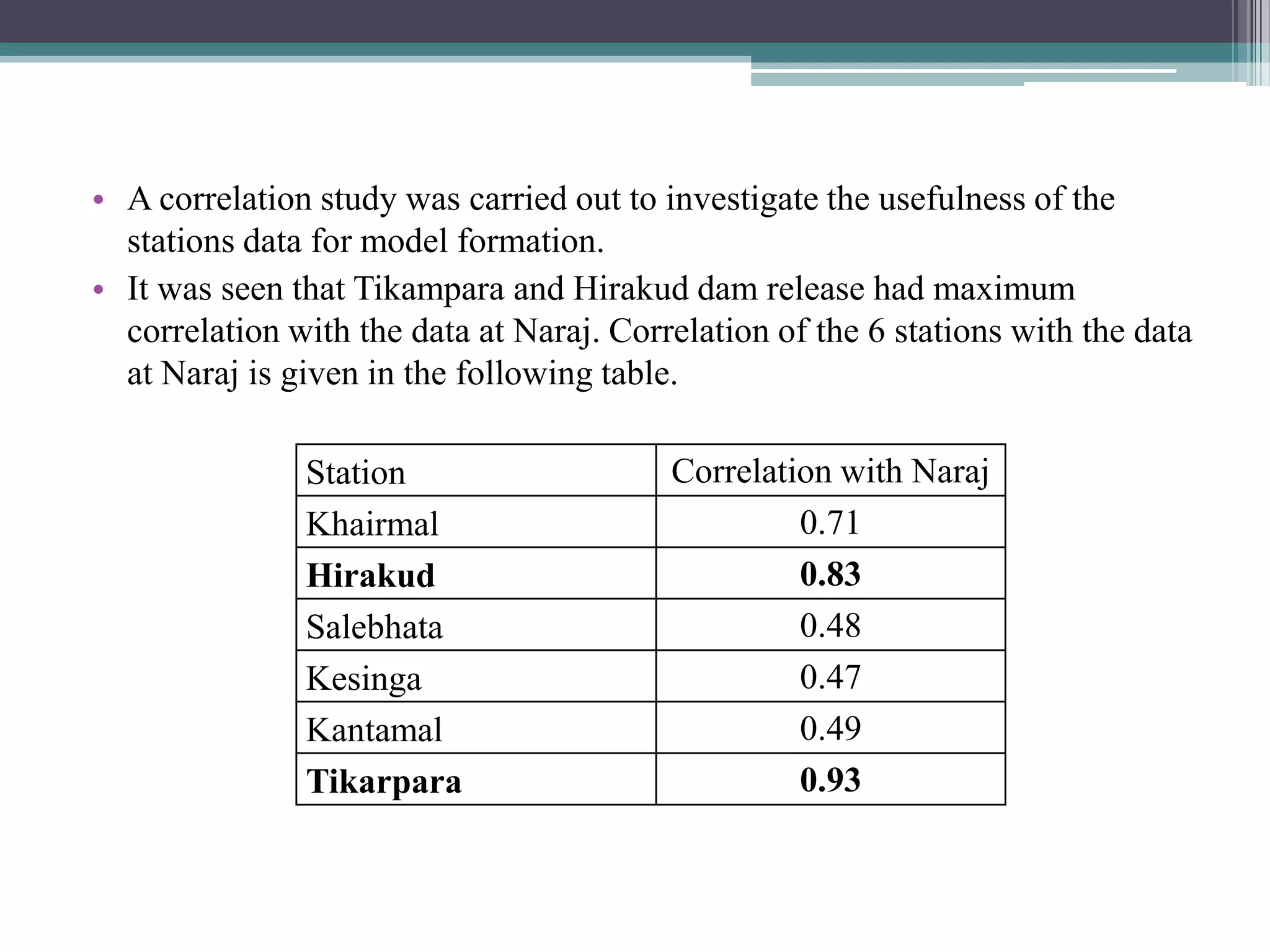
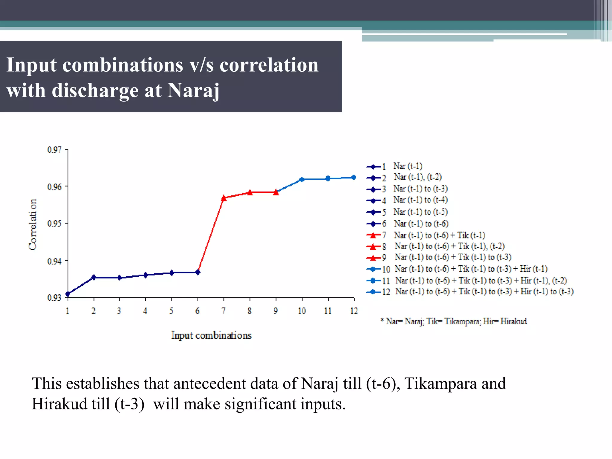
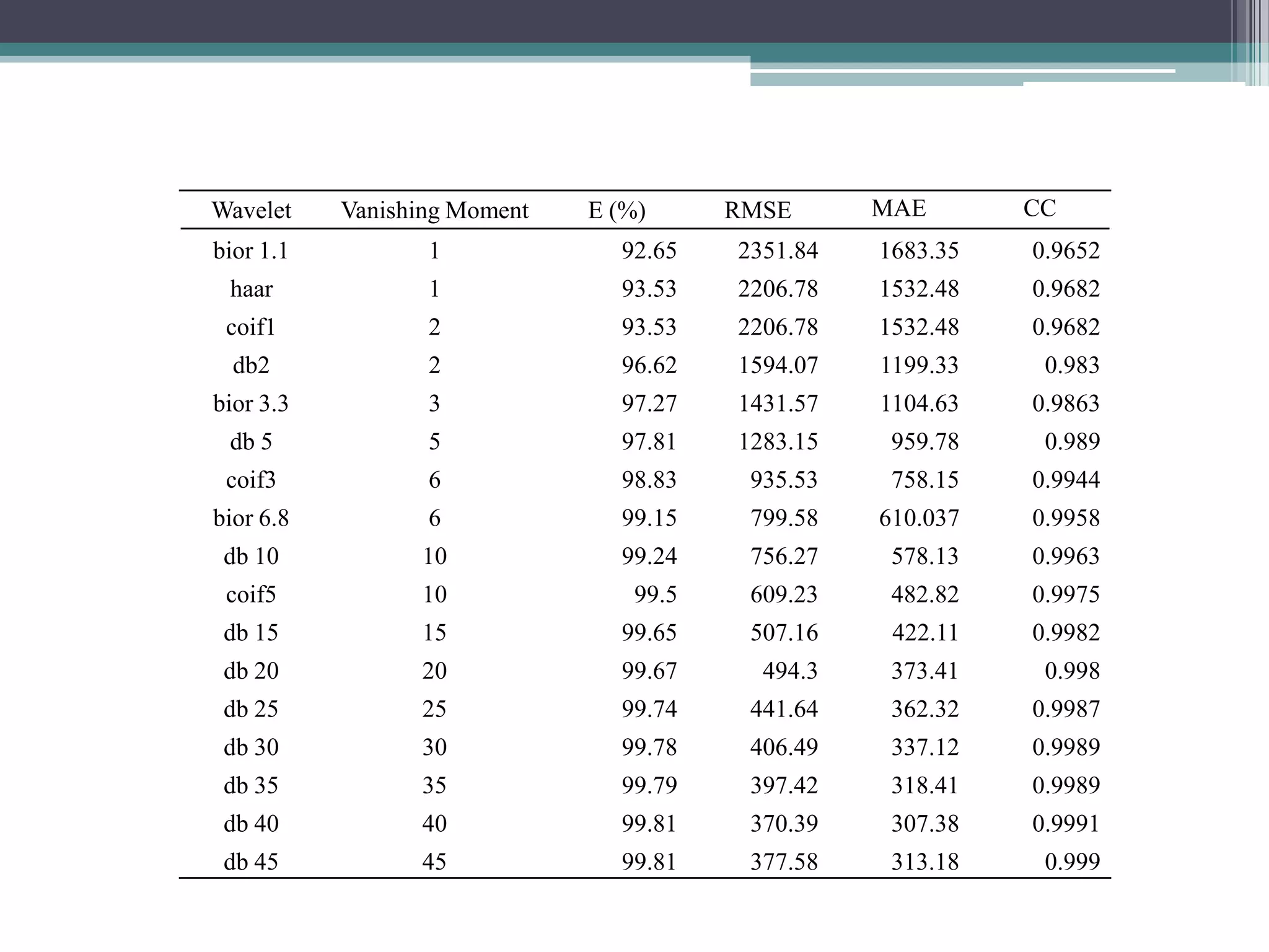
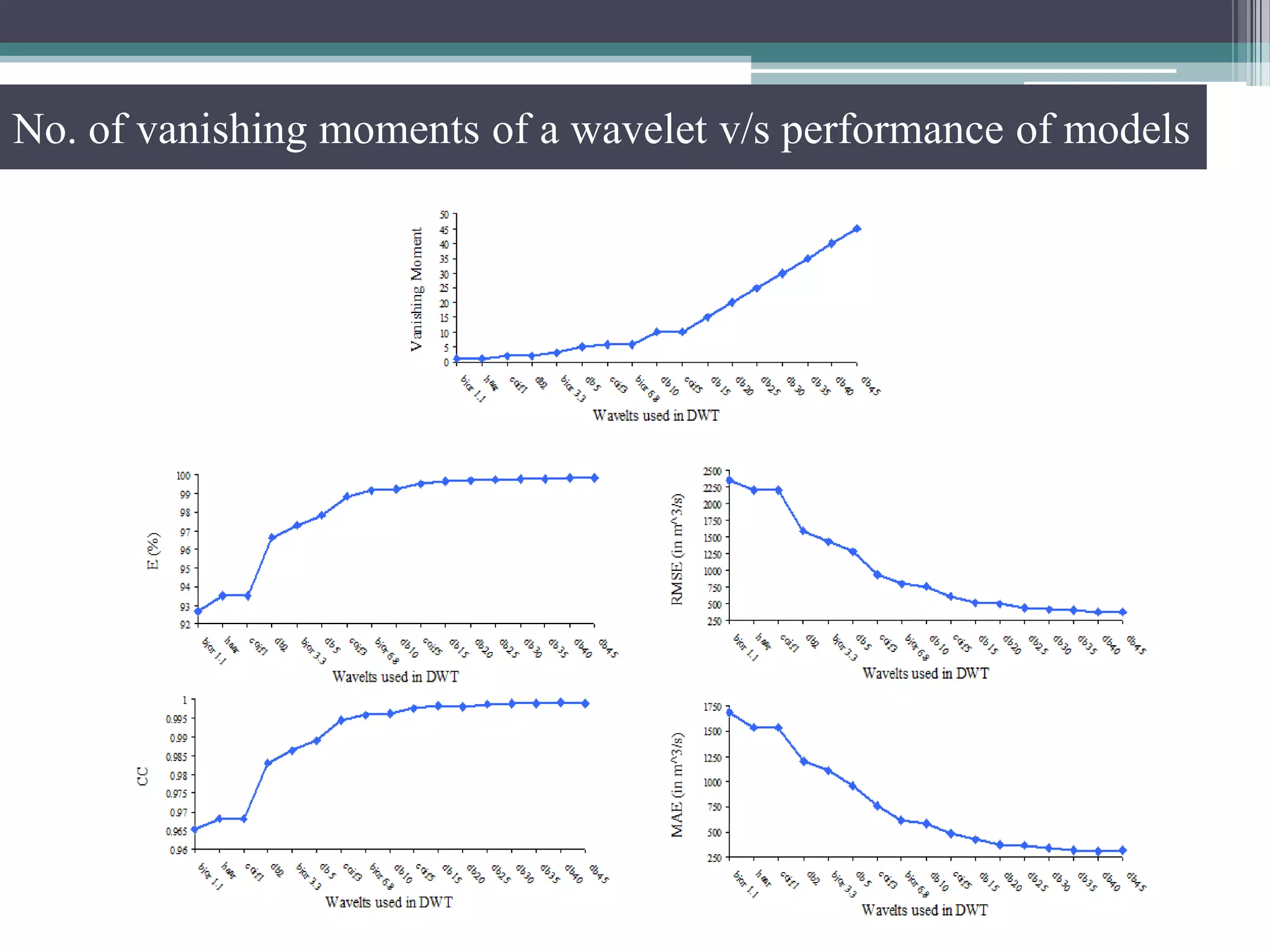
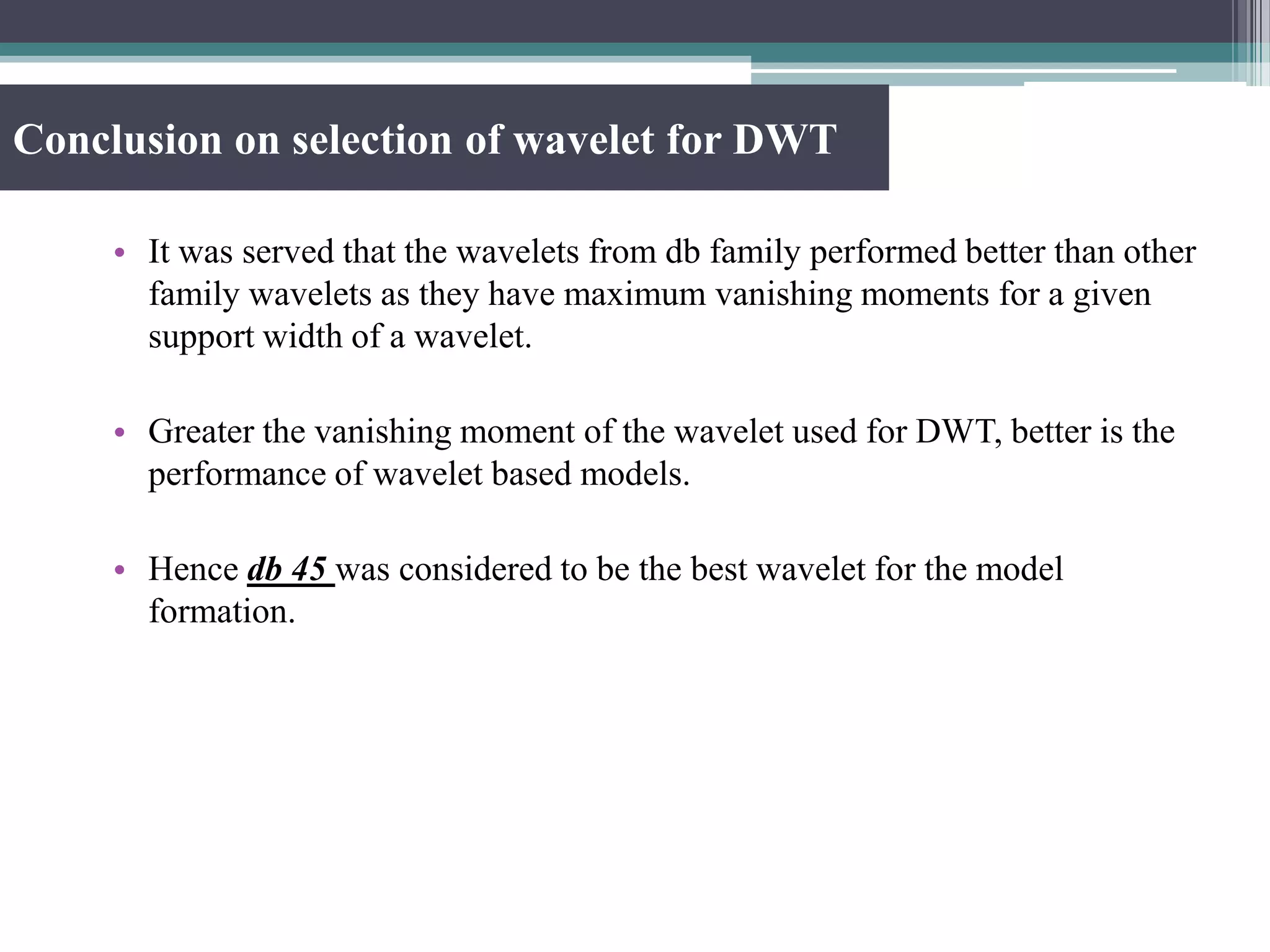
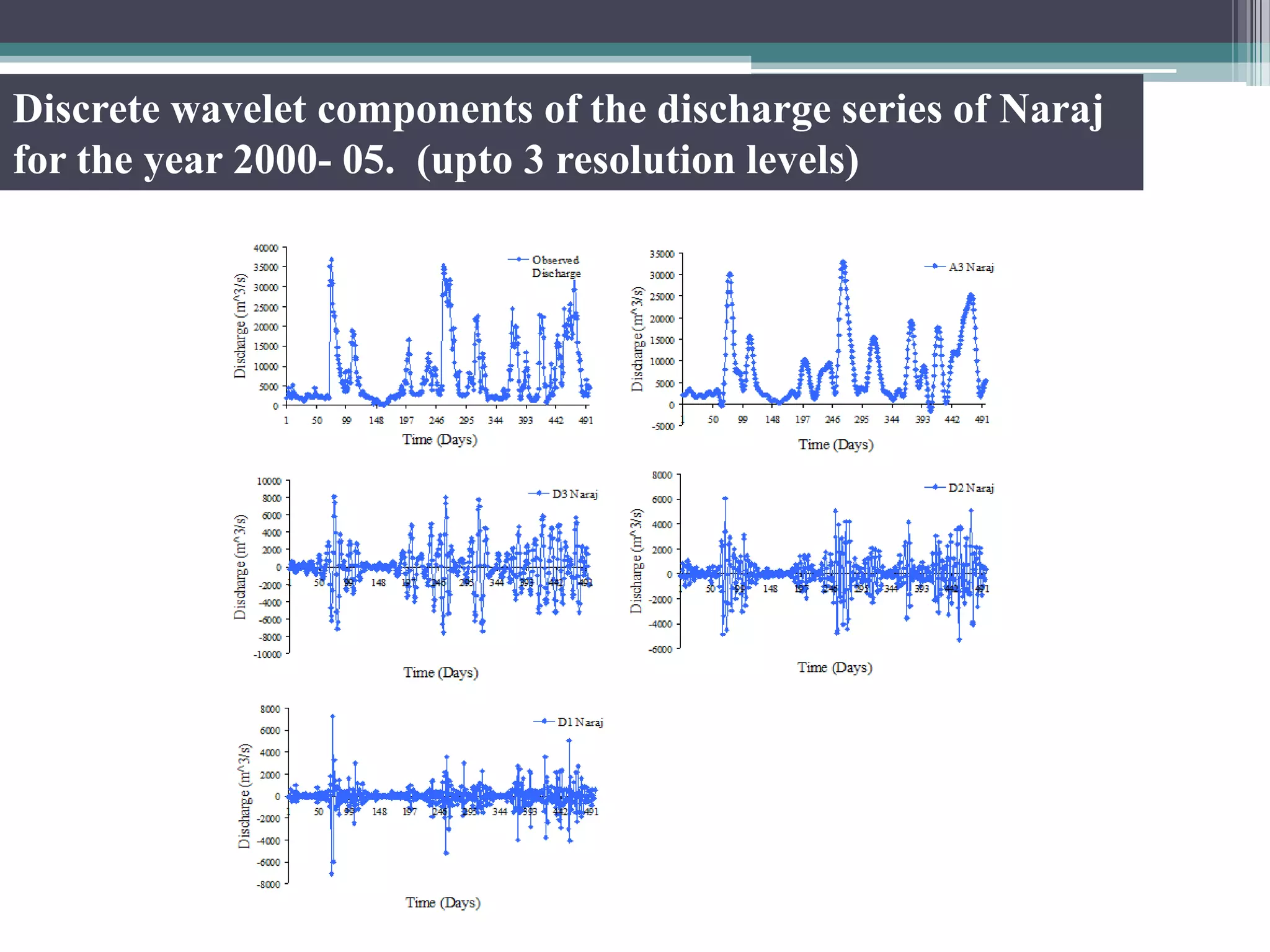
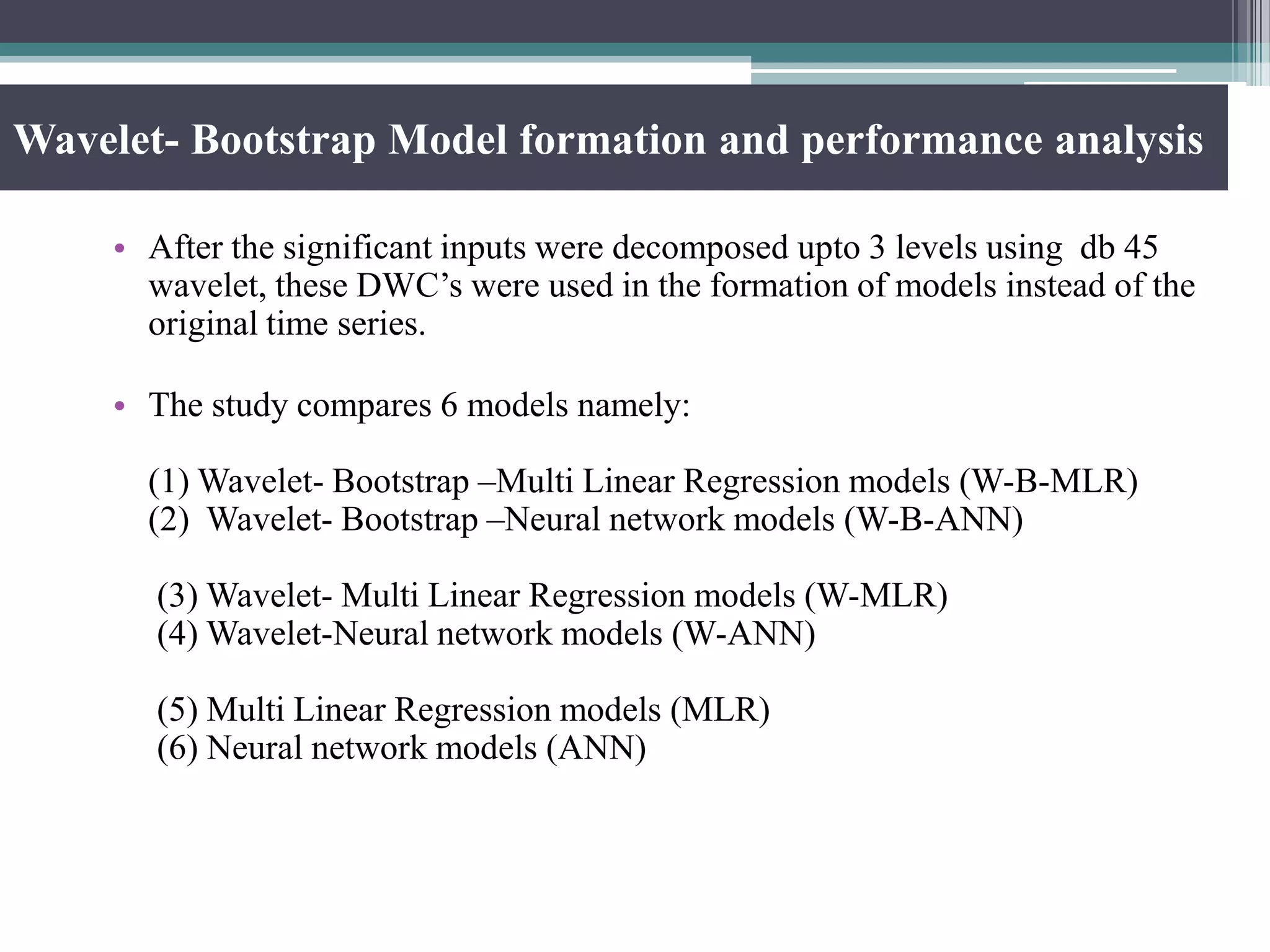
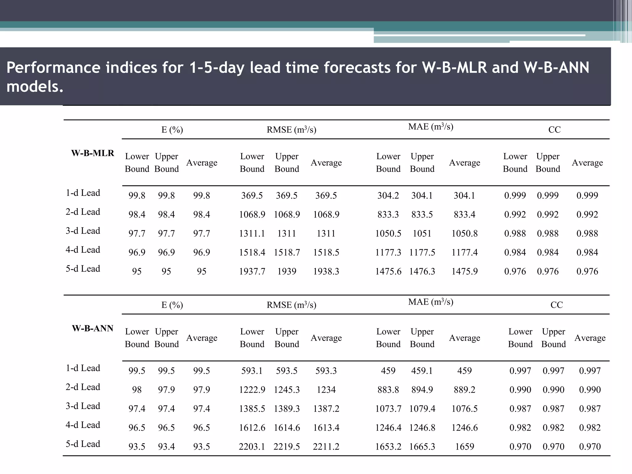
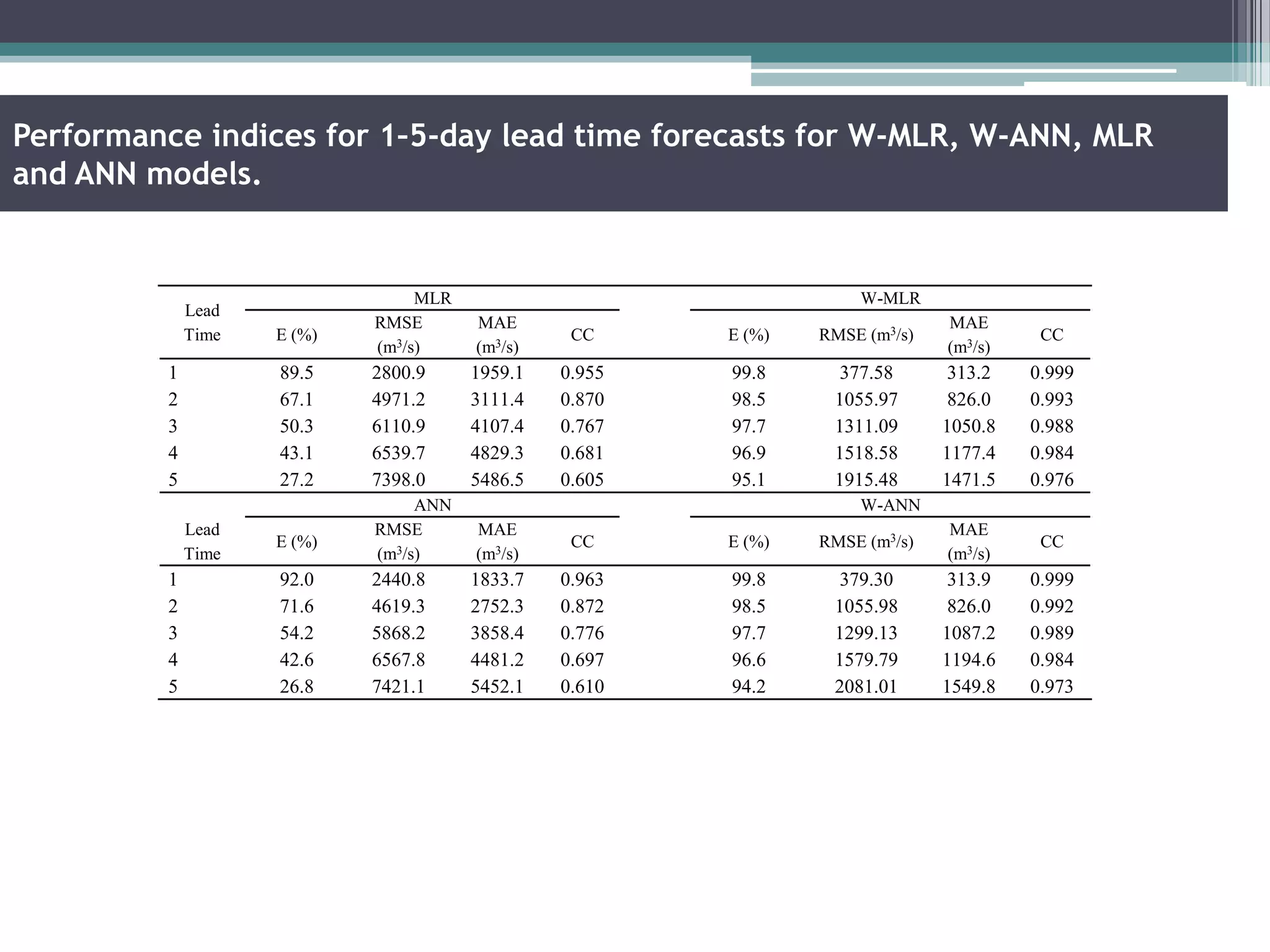
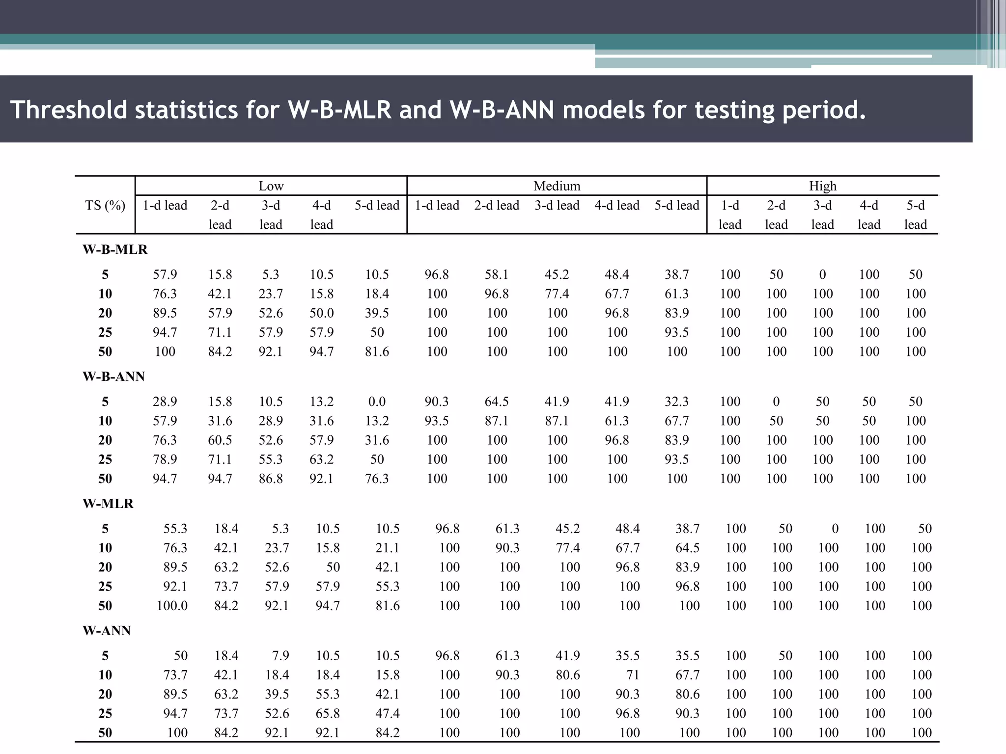
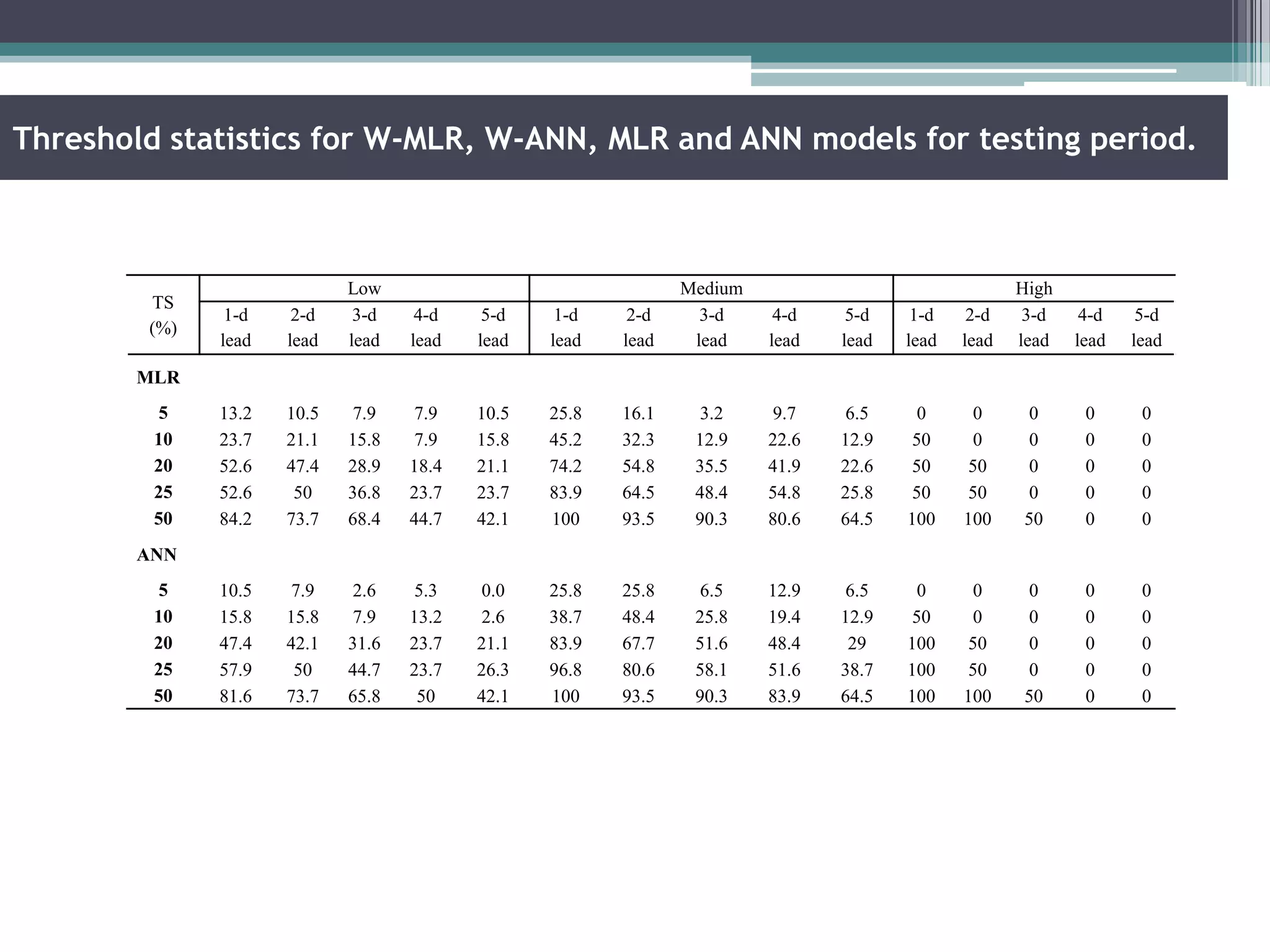
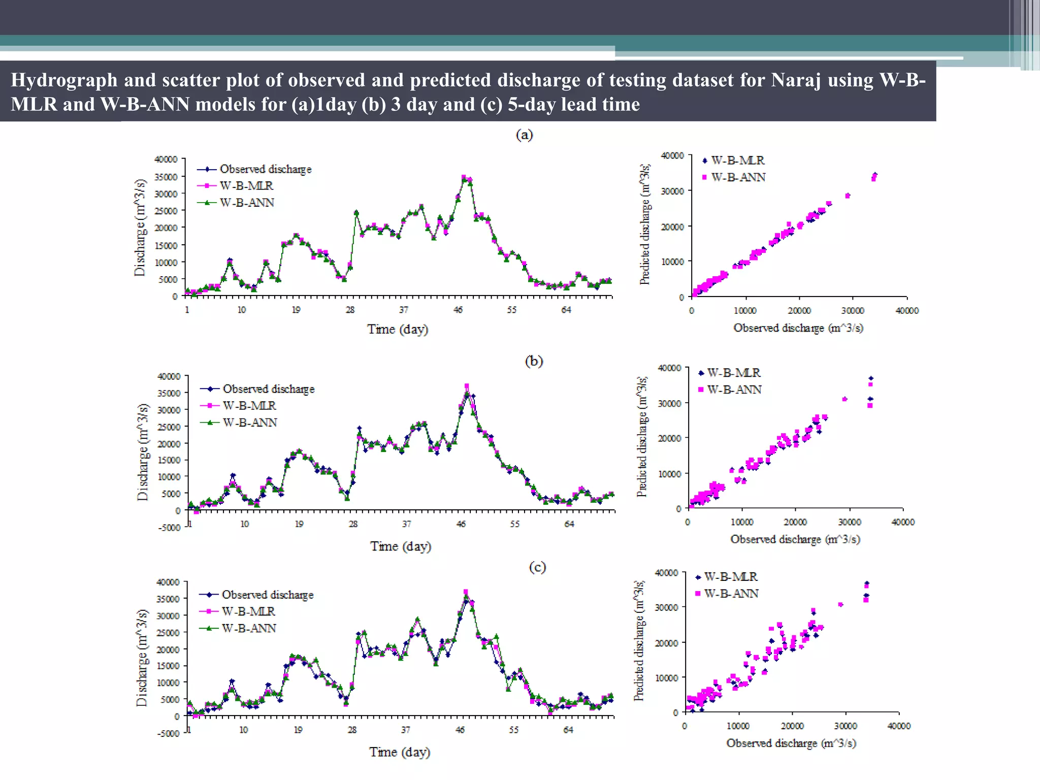
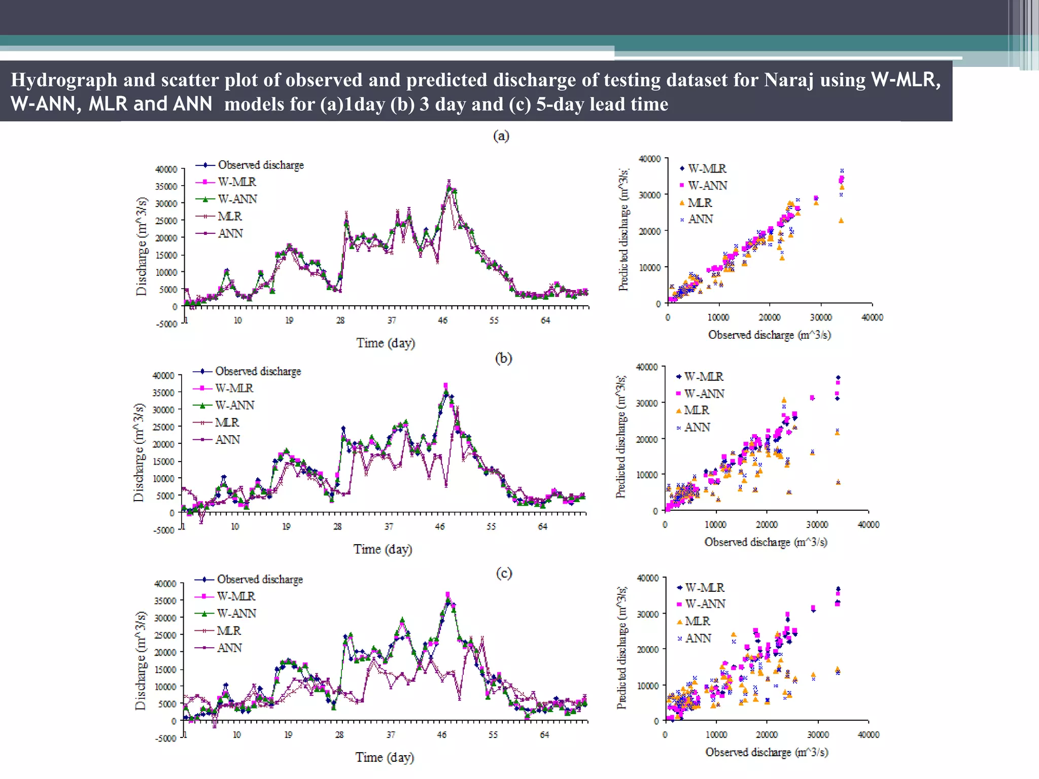
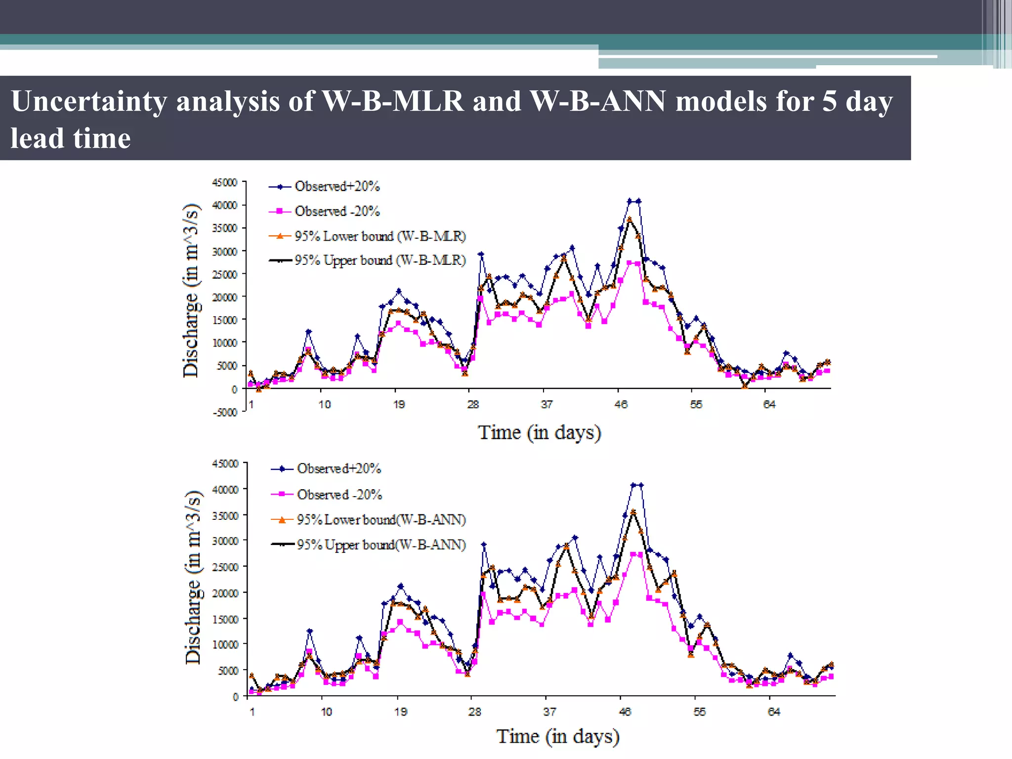
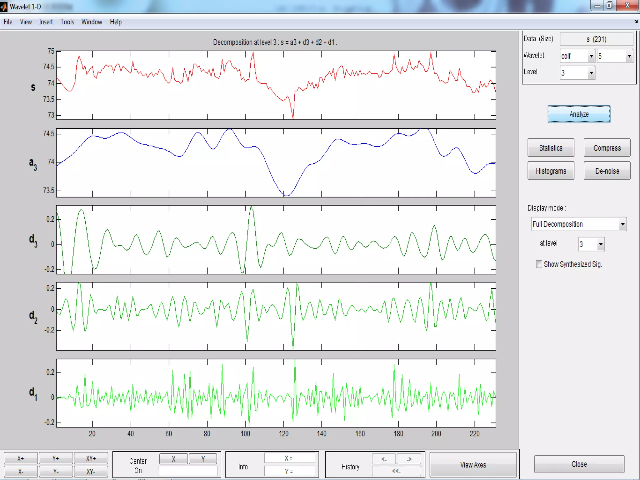
Wavelet - Bootstrap based Multiple
linear regression models for flood
forecasting in Mahanadi basin.
- Vinit Sehgal Under The guidance of:
4th year UG Student Dr. C. Chatterjee
Department Of Civil Engineering Agril. & Food Engg. Department
Birla Institute of Technology Indian Institute of Technology
Mesra, Ranchi Kharagpur
Problem statement
• The aim of the study was to
(a) develop accurate and reliable models for daily discharge forecasting
based on Wavelet and bootstrap soft computing techniques using the
minimum possible data and
(b) to compare the results with the previous studies on the Mahanadi basin.
I
Catchment area and
Selection of Data
• Data sets for seven stations of Mahanadi basins were
available, namely, Naraj, Tikampara, Khairmal, Kantamal, Kesingha, Saleb
hata and Hirakud dam which are shown in the figure.
• A correlation study was carried out to investigate the usefulness of the
stations data for model formation.
• It was seen that Tikampara and Hirakud dam release had maximum
correlation with the data at Naraj. Correlation of the 6 stations with the data
at Naraj is given in the following table.
Station Correlation with Naraj
Khairmal 0.71
Hirakud 0.83
Salebhata 0.48
Kesinga 0.47
Kantamal 0.49
Tikarpara 0.93
• Only discharge at Tikampara and Hirakud release were found to be in good
correlation with the discharge at Naraj.
• Further correlation analysis showed that keeping other stations in the
model formation wont help improve the results (results not shown).
• The correlation study was extended further to decide the significant
antecedent time series from each station in the formation of models.
Input combinations v/s correlation
with discharge at Naraj
This establishes that antecedent data of Naraj till (t-6), Tikampara and
Hirakud till (t-3) will make significant inputs.
II
Selection of Wavelet for DWT
• Selection of wavelets if an important factor on which the performance of
wavelet based models depend.
• Wavelets with high vanishing moments are believed to be more sensitive
towards high frequencies, and hence, are more suitable for application in
hydrological forecasting problems.
• A novel study was carried out in which wavelet based simple MLR models
were formed using 17 wavelets of various families to forecast 1- day ahead
discharge at Naraj using the DWC’s of the significant inputs as described
in slide 6 and the results were tabulated as follows.
Wavelet Vanishing Moment E (%) RMSE MAE CC
bior 1.1 1 92.65 2351.84 1683.35 0.9652
haar 1 93.53 2206.78 1532.48 0.9682
coif1 2 93.53 2206.78 1532.48 0.9682
db2 2 96.62 1594.07 1199.33 0.983
bior 3.3 3 97.27 1431.57 1104.63 0.9863
db 5 5 97.81 1283.15 959.78 0.989
coif3 6 98.83 935.53 758.15 0.9944
bior 6.8 6 99.15 799.58 610.037 0.9958
db 10 10 99.24 756.27 578.13 0.9963
coif5 10 99.5 609.23 482.82 0.9975
db 15 15 99.65 507.16 422.11 0.9982
db 20 20 99.67 494.3 373.41 0.998
db 25 25 99.74 441.64 362.32 0.9987
db 30 30 99.78 406.49 337.12 0.9989
db 35 35 99.79 397.42 318.41 0.9989
db 40 40 99.81 370.39 307.38 0.9991
db 45 45 99.81 377.58 313.18 0.999
No. of vanishing moments of a wavelet v/s performance of models
Conclusion on selection of wavelet for DWT
• It was served that the wavelets from db family performed better than other
family wavelets as they have maximum vanishing moments for a given
support width of a wavelet.
• Greater the vanishing moment of the wavelet used for DWT, better is the
performance of wavelet based models.
• Hence db 45 was considered to be the best wavelet for the model
formation.
Discrete wavelet components of the discharge series of Naraj
for the year 2000- 05. (upto 3 resolution levels)
III
Wavelet- Bootstrap Model formation and performance analysis
• After the significant inputs were decomposed upto 3 levels using db 45
wavelet, these DWC’s were used in the formation of models instead of the
original time series.
• The study compares 6 models namely:
(1) Wavelet- Bootstrap –Multi Linear Regression models (W-B-MLR)
(2) Wavelet- Bootstrap –Neural network models (W-B-ANN)
(3) Wavelet- Multi Linear Regression models (W-MLR)
(4) Wavelet-Neural network models (W-ANN)
(5) Multi Linear Regression models (MLR)
(6) Neural network models (ANN)
Performance indices for 1–5-day lead time forecasts for W-B-MLR and W-B-ANN
models.
W-B-MLR
E (%) RMSE (m3/s) MAE (m3/s) CC
Lower
Bound
Upper
Bound
Average
Lower
Bound
Upper
Bound
Average
Lower
Bound
Upper
Bound
Average
Lower
Bound
Upper
Bound
Average
1-d Lead 99.8 99.8 99.8 369.5 369.5 369.5 304.2 304.1 304.1 0.999 0.999 0.999
2-d Lead 98.4 98.4 98.4 1068.9 1068.9 1068.9 833.3 833.5 833.4 0.992 0.992 0.992
3-d Lead 97.7 97.7 97.7 1311.1 1311 1311 1050.5 1051 1050.8 0.988 0.988 0.988
4-d Lead 96.9 96.9 96.9 1518.4 1518.7 1518.5 1177.3 1177.5 1177.4 0.984 0.984 0.984
5-d Lead 95 95 95 1937.7 1939 1938.3 1475.6 1476.3 1475.9 0.976 0.976 0.976
W-B-ANN
E (%) RMSE (m3/s) MAE (m3/s) CC
Lower
Bound
Upper
Bound
Average
Lower
Bound
Upper
Bound
Average
Lower
Bound
Upper
Bound
Average
Lower
Bound
Upper
Bound
Average
1-d Lead 99.5 99.5 99.5 593.1 593.5 593.3 459 459.1 459 0.997 0.997 0.997
2-d Lead 98 97.9 97.9 1222.9 1245.3 1234 883.8 894.9 889.2 0.990 0.990 0.990
3-d Lead 97.4 97.4 97.4 1385.5 1389.3 1387.2 1073.7 1079.4 1076.5 0.987 0.987 0.987
4-d Lead 96.5 96.5 96.5 1612.6 1614.6 1613.4 1246.4 1246.8 1246.6 0.982 0.982 0.982
5-d Lead 93.5 93.4 93.5 2203.1 2219.5 2211.2 1653.2 1665.3 1659 0.970 0.970 0.970
Performance indices for 1–5-day lead time forecasts for W-MLR, W-ANN, MLR
and ANN models.
Lead
Time
MLR W-MLR
E (%)
RMSE
(m3/s)
MAE
(m3/s)
CC E (%) RMSE (m3/s)
MAE
(m3/s)
CC
1 89.5 2800.9 1959.1 0.955 99.8 377.58 313.2 0.999
2 67.1 4971.2 3111.4 0.870 98.5 1055.97 826.0 0.993
3 50.3 6110.9 4107.4 0.767 97.7 1311.09 1050.8 0.988
4 43.1 6539.7 4829.3 0.681 96.9 1518.58 1177.4 0.984
5 27.2 7398.0 5486.5 0.605 95.1 1915.48 1471.5 0.976
Lead
Time
ANN W-ANN
E (%)
RMSE
(m3/s)
MAE
(m3/s)
CC E (%) RMSE (m3/s)
MAE
(m3/s)
CC
1 92.0 2440.8 1833.7 0.963 99.8 379.30 313.9 0.999
2 71.6 4619.3 2752.3 0.872 98.5 1055.98 826.0 0.992
3 54.2 5868.2 3858.4 0.776 97.7 1299.13 1087.2 0.989
4 42.6 6567.8 4481.2 0.697 96.6 1579.79 1194.6 0.984
5 26.8 7421.1 5452.1 0.610 94.2 2081.01 1549.8 0.973
Threshold statistics for W-B-MLR and W-B-ANN models for testing period.
TS (%)
Low Medium High
1-d lead 2-d
lead
3-d
lead
4-d
lead
5-d lead 1-d lead 2-d lead 3-d lead 4-d lead 5-d lead 1-d
lead
2-d
lead
3-d
lead
4-d
lead
5-d
lead
W-B-MLR
5 57.9 15.8 5.3 10.5 10.5 96.8 58.1 45.2 48.4 38.7 100 50 0 100 50
10 76.3 42.1 23.7 15.8 18.4 100 96.8 77.4 67.7 61.3 100 100 100 100 100
20 89.5 57.9 52.6 50.0 39.5 100 100 100 96.8 83.9 100 100 100 100 100
25 94.7 71.1 57.9 57.9 50 100 100 100 100 93.5 100 100 100 100 100
50 100 84.2 92.1 94.7 81.6 100 100 100 100 100 100 100 100 100 100
W-B-ANN
5 28.9 15.8 10.5 13.2 0.0 90.3 64.5 41.9 41.9 32.3 100 0 50 50 50
10 57.9 31.6 28.9 31.6 13.2 93.5 87.1 87.1 61.3 67.7 100 50 50 50 100
20 76.3 60.5 52.6 57.9 31.6 100 100 100 96.8 83.9 100 100 100 100 100
25 78.9 71.1 55.3 63.2 50 100 100 100 100 93.5 100 100 100 100 100
50 94.7 94.7 86.8 92.1 76.3 100 100 100 100 100 100 100 100 100 100
W-MLR
5 55.3 18.4 5.3 10.5 10.5 96.8 61.3 45.2 48.4 38.7 100 50 0 100 50
10 76.3 42.1 23.7 15.8 21.1 100 90.3 77.4 67.7 64.5 100 100 100 100 100
20 89.5 63.2 52.6 50 42.1 100 100 100 96.8 83.9 100 100 100 100 100
25 92.1 73.7 57.9 57.9 55.3 100 100 100 100 96.8 100 100 100 100 100
50 100.0 84.2 92.1 94.7 81.6 100 100 100 100 100 100 100 100 100 100
W-ANN
5 50 18.4 7.9 10.5 10.5 96.8 61.3 41.9 35.5 35.5 100 50 100 100 100
10 73.7 42.1 18.4 18.4 15.8 100 90.3 80.6 71 67.7 100 100 100 100 100
20 89.5 63.2 39.5 55.3 42.1 100 100 100 90.3 80.6 100 100 100 100 100
25 94.7 73.7 52.6 65.8 47.4 100 100 100 96.8 90.3 100 100 100 100 100
50 100 84.2 92.1 92.1 84.2 100 100 100 100 100 100 100 100 100 100
Threshold statistics for W-MLR, W-ANN, MLR and ANN models for testing period.
TS
(%)
Low Medium High
1-d
lead
2-d
lead
3-d
lead
4-d
lead
5-d
lead
1-d
lead
2-d
lead
3-d
lead
4-d
lead
5-d
lead
1-d
lead
2-d
lead
3-d
lead
4-d
lead
5-d
lead
MLR
5 13.2 10.5 7.9 7.9 10.5 25.8 16.1 3.2 9.7 6.5 0 0 0 0 0
10 23.7 21.1 15.8 7.9 15.8 45.2 32.3 12.9 22.6 12.9 50 0 0 0 0
20 52.6 47.4 28.9 18.4 21.1 74.2 54.8 35.5 41.9 22.6 50 50 0 0 0
25 52.6 50 36.8 23.7 23.7 83.9 64.5 48.4 54.8 25.8 50 50 0 0 0
50 84.2 73.7 68.4 44.7 42.1 100 93.5 90.3 80.6 64.5 100 100 50 0 0
ANN
5 10.5 7.9 2.6 5.3 0.0 25.8 25.8 6.5 12.9 6.5 0 0 0 0 0
10 15.8 15.8 7.9 13.2 2.6 38.7 48.4 25.8 19.4 12.9 50 0 0 0 0
20 47.4 42.1 31.6 23.7 21.1 83.9 67.7 51.6 48.4 29 100 50 0 0 0
25 57.9 50 44.7 23.7 26.3 96.8 80.6 58.1 51.6 38.7 100 50 0 0 0
50 81.6 73.7 65.8 50 42.1 100 93.5 90.3 83.9 64.5 100 100 50 0 0
Hydrograph and scatter plot of observed and predicted discharge of testing dataset for Naraj using W-B-
MLR and W-B-ANN models for (a)1day (b) 3 day and (c) 5-day lead time
Hydrograph and scatter plot of observed and predicted discharge of testing dataset for Naraj using W-MLR,
W-ANN, MLR and ANN models for (a)1day (b) 3 day and (c) 5-day lead time
Uncertainty analysis
• CWC suggests that 20 % (plus or minus) error in forecasting discharge is
acceptable. So the pattern of the 95% upper and lower bands of the
predictions using Bootstrap methods was studied with respect to the 20%
upper and lower band of the original discharge at Naraj.
Uncertainty analysis of W-B-MLR and W-B-ANN models for 5 day
lead time
Wavelet bootstrap Multiple linear regression models

Wavelet bootstrap Multiple linear regression models

  • 1.
    Wavelet - Bootstrapbased Multiple linear regression models for flood forecasting in Mahanadi basin. - Vinit Sehgal Under The guidance of: 4th year UG Student Dr. C. Chatterjee Department Of Civil Engineering Agril. & Food Engg. Department Birla Institute of Technology Indian Institute of Technology Mesra, Ranchi Kharagpur
  • 2.
    Problem statement • Theaim of the study was to (a) develop accurate and reliable models for daily discharge forecasting based on Wavelet and bootstrap soft computing techniques using the minimum possible data and (b) to compare the results with the previous studies on the Mahanadi basin.
  • 3.
  • 4.
    Catchment area and Selectionof Data • Data sets for seven stations of Mahanadi basins were available, namely, Naraj, Tikampara, Khairmal, Kantamal, Kesingha, Saleb hata and Hirakud dam which are shown in the figure.
  • 5.
    • A correlationstudy was carried out to investigate the usefulness of the stations data for model formation. • It was seen that Tikampara and Hirakud dam release had maximum correlation with the data at Naraj. Correlation of the 6 stations with the data at Naraj is given in the following table. Station Correlation with Naraj Khairmal 0.71 Hirakud 0.83 Salebhata 0.48 Kesinga 0.47 Kantamal 0.49 Tikarpara 0.93
  • 6.
    • Only dischargeat Tikampara and Hirakud release were found to be in good correlation with the discharge at Naraj. • Further correlation analysis showed that keeping other stations in the model formation wont help improve the results (results not shown). • The correlation study was extended further to decide the significant antecedent time series from each station in the formation of models.
  • 7.
    Input combinations v/scorrelation with discharge at Naraj This establishes that antecedent data of Naraj till (t-6), Tikampara and Hirakud till (t-3) will make significant inputs.
  • 8.
  • 9.
    Selection of Waveletfor DWT • Selection of wavelets if an important factor on which the performance of wavelet based models depend. • Wavelets with high vanishing moments are believed to be more sensitive towards high frequencies, and hence, are more suitable for application in hydrological forecasting problems. • A novel study was carried out in which wavelet based simple MLR models were formed using 17 wavelets of various families to forecast 1- day ahead discharge at Naraj using the DWC’s of the significant inputs as described in slide 6 and the results were tabulated as follows.
  • 10.
    Wavelet Vanishing MomentE (%) RMSE MAE CC bior 1.1 1 92.65 2351.84 1683.35 0.9652 haar 1 93.53 2206.78 1532.48 0.9682 coif1 2 93.53 2206.78 1532.48 0.9682 db2 2 96.62 1594.07 1199.33 0.983 bior 3.3 3 97.27 1431.57 1104.63 0.9863 db 5 5 97.81 1283.15 959.78 0.989 coif3 6 98.83 935.53 758.15 0.9944 bior 6.8 6 99.15 799.58 610.037 0.9958 db 10 10 99.24 756.27 578.13 0.9963 coif5 10 99.5 609.23 482.82 0.9975 db 15 15 99.65 507.16 422.11 0.9982 db 20 20 99.67 494.3 373.41 0.998 db 25 25 99.74 441.64 362.32 0.9987 db 30 30 99.78 406.49 337.12 0.9989 db 35 35 99.79 397.42 318.41 0.9989 db 40 40 99.81 370.39 307.38 0.9991 db 45 45 99.81 377.58 313.18 0.999
  • 11.
    No. of vanishingmoments of a wavelet v/s performance of models
  • 12.
    Conclusion on selectionof wavelet for DWT • It was served that the wavelets from db family performed better than other family wavelets as they have maximum vanishing moments for a given support width of a wavelet. • Greater the vanishing moment of the wavelet used for DWT, better is the performance of wavelet based models. • Hence db 45 was considered to be the best wavelet for the model formation.
  • 13.
    Discrete wavelet componentsof the discharge series of Naraj for the year 2000- 05. (upto 3 resolution levels)
  • 14.
  • 15.
    Wavelet- Bootstrap Modelformation and performance analysis • After the significant inputs were decomposed upto 3 levels using db 45 wavelet, these DWC’s were used in the formation of models instead of the original time series. • The study compares 6 models namely: (1) Wavelet- Bootstrap –Multi Linear Regression models (W-B-MLR) (2) Wavelet- Bootstrap –Neural network models (W-B-ANN) (3) Wavelet- Multi Linear Regression models (W-MLR) (4) Wavelet-Neural network models (W-ANN) (5) Multi Linear Regression models (MLR) (6) Neural network models (ANN)
  • 16.
    Performance indices for1–5-day lead time forecasts for W-B-MLR and W-B-ANN models. W-B-MLR E (%) RMSE (m3/s) MAE (m3/s) CC Lower Bound Upper Bound Average Lower Bound Upper Bound Average Lower Bound Upper Bound Average Lower Bound Upper Bound Average 1-d Lead 99.8 99.8 99.8 369.5 369.5 369.5 304.2 304.1 304.1 0.999 0.999 0.999 2-d Lead 98.4 98.4 98.4 1068.9 1068.9 1068.9 833.3 833.5 833.4 0.992 0.992 0.992 3-d Lead 97.7 97.7 97.7 1311.1 1311 1311 1050.5 1051 1050.8 0.988 0.988 0.988 4-d Lead 96.9 96.9 96.9 1518.4 1518.7 1518.5 1177.3 1177.5 1177.4 0.984 0.984 0.984 5-d Lead 95 95 95 1937.7 1939 1938.3 1475.6 1476.3 1475.9 0.976 0.976 0.976 W-B-ANN E (%) RMSE (m3/s) MAE (m3/s) CC Lower Bound Upper Bound Average Lower Bound Upper Bound Average Lower Bound Upper Bound Average Lower Bound Upper Bound Average 1-d Lead 99.5 99.5 99.5 593.1 593.5 593.3 459 459.1 459 0.997 0.997 0.997 2-d Lead 98 97.9 97.9 1222.9 1245.3 1234 883.8 894.9 889.2 0.990 0.990 0.990 3-d Lead 97.4 97.4 97.4 1385.5 1389.3 1387.2 1073.7 1079.4 1076.5 0.987 0.987 0.987 4-d Lead 96.5 96.5 96.5 1612.6 1614.6 1613.4 1246.4 1246.8 1246.6 0.982 0.982 0.982 5-d Lead 93.5 93.4 93.5 2203.1 2219.5 2211.2 1653.2 1665.3 1659 0.970 0.970 0.970
  • 17.
    Performance indices for1–5-day lead time forecasts for W-MLR, W-ANN, MLR and ANN models. Lead Time MLR W-MLR E (%) RMSE (m3/s) MAE (m3/s) CC E (%) RMSE (m3/s) MAE (m3/s) CC 1 89.5 2800.9 1959.1 0.955 99.8 377.58 313.2 0.999 2 67.1 4971.2 3111.4 0.870 98.5 1055.97 826.0 0.993 3 50.3 6110.9 4107.4 0.767 97.7 1311.09 1050.8 0.988 4 43.1 6539.7 4829.3 0.681 96.9 1518.58 1177.4 0.984 5 27.2 7398.0 5486.5 0.605 95.1 1915.48 1471.5 0.976 Lead Time ANN W-ANN E (%) RMSE (m3/s) MAE (m3/s) CC E (%) RMSE (m3/s) MAE (m3/s) CC 1 92.0 2440.8 1833.7 0.963 99.8 379.30 313.9 0.999 2 71.6 4619.3 2752.3 0.872 98.5 1055.98 826.0 0.992 3 54.2 5868.2 3858.4 0.776 97.7 1299.13 1087.2 0.989 4 42.6 6567.8 4481.2 0.697 96.6 1579.79 1194.6 0.984 5 26.8 7421.1 5452.1 0.610 94.2 2081.01 1549.8 0.973
  • 18.
    Threshold statistics forW-B-MLR and W-B-ANN models for testing period. TS (%) Low Medium High 1-d lead 2-d lead 3-d lead 4-d lead 5-d lead 1-d lead 2-d lead 3-d lead 4-d lead 5-d lead 1-d lead 2-d lead 3-d lead 4-d lead 5-d lead W-B-MLR 5 57.9 15.8 5.3 10.5 10.5 96.8 58.1 45.2 48.4 38.7 100 50 0 100 50 10 76.3 42.1 23.7 15.8 18.4 100 96.8 77.4 67.7 61.3 100 100 100 100 100 20 89.5 57.9 52.6 50.0 39.5 100 100 100 96.8 83.9 100 100 100 100 100 25 94.7 71.1 57.9 57.9 50 100 100 100 100 93.5 100 100 100 100 100 50 100 84.2 92.1 94.7 81.6 100 100 100 100 100 100 100 100 100 100 W-B-ANN 5 28.9 15.8 10.5 13.2 0.0 90.3 64.5 41.9 41.9 32.3 100 0 50 50 50 10 57.9 31.6 28.9 31.6 13.2 93.5 87.1 87.1 61.3 67.7 100 50 50 50 100 20 76.3 60.5 52.6 57.9 31.6 100 100 100 96.8 83.9 100 100 100 100 100 25 78.9 71.1 55.3 63.2 50 100 100 100 100 93.5 100 100 100 100 100 50 94.7 94.7 86.8 92.1 76.3 100 100 100 100 100 100 100 100 100 100 W-MLR 5 55.3 18.4 5.3 10.5 10.5 96.8 61.3 45.2 48.4 38.7 100 50 0 100 50 10 76.3 42.1 23.7 15.8 21.1 100 90.3 77.4 67.7 64.5 100 100 100 100 100 20 89.5 63.2 52.6 50 42.1 100 100 100 96.8 83.9 100 100 100 100 100 25 92.1 73.7 57.9 57.9 55.3 100 100 100 100 96.8 100 100 100 100 100 50 100.0 84.2 92.1 94.7 81.6 100 100 100 100 100 100 100 100 100 100 W-ANN 5 50 18.4 7.9 10.5 10.5 96.8 61.3 41.9 35.5 35.5 100 50 100 100 100 10 73.7 42.1 18.4 18.4 15.8 100 90.3 80.6 71 67.7 100 100 100 100 100 20 89.5 63.2 39.5 55.3 42.1 100 100 100 90.3 80.6 100 100 100 100 100 25 94.7 73.7 52.6 65.8 47.4 100 100 100 96.8 90.3 100 100 100 100 100 50 100 84.2 92.1 92.1 84.2 100 100 100 100 100 100 100 100 100 100
  • 19.
    Threshold statistics forW-MLR, W-ANN, MLR and ANN models for testing period. TS (%) Low Medium High 1-d lead 2-d lead 3-d lead 4-d lead 5-d lead 1-d lead 2-d lead 3-d lead 4-d lead 5-d lead 1-d lead 2-d lead 3-d lead 4-d lead 5-d lead MLR 5 13.2 10.5 7.9 7.9 10.5 25.8 16.1 3.2 9.7 6.5 0 0 0 0 0 10 23.7 21.1 15.8 7.9 15.8 45.2 32.3 12.9 22.6 12.9 50 0 0 0 0 20 52.6 47.4 28.9 18.4 21.1 74.2 54.8 35.5 41.9 22.6 50 50 0 0 0 25 52.6 50 36.8 23.7 23.7 83.9 64.5 48.4 54.8 25.8 50 50 0 0 0 50 84.2 73.7 68.4 44.7 42.1 100 93.5 90.3 80.6 64.5 100 100 50 0 0 ANN 5 10.5 7.9 2.6 5.3 0.0 25.8 25.8 6.5 12.9 6.5 0 0 0 0 0 10 15.8 15.8 7.9 13.2 2.6 38.7 48.4 25.8 19.4 12.9 50 0 0 0 0 20 47.4 42.1 31.6 23.7 21.1 83.9 67.7 51.6 48.4 29 100 50 0 0 0 25 57.9 50 44.7 23.7 26.3 96.8 80.6 58.1 51.6 38.7 100 50 0 0 0 50 81.6 73.7 65.8 50 42.1 100 93.5 90.3 83.9 64.5 100 100 50 0 0
  • 20.
    Hydrograph and scatterplot of observed and predicted discharge of testing dataset for Naraj using W-B- MLR and W-B-ANN models for (a)1day (b) 3 day and (c) 5-day lead time
  • 21.
    Hydrograph and scatterplot of observed and predicted discharge of testing dataset for Naraj using W-MLR, W-ANN, MLR and ANN models for (a)1day (b) 3 day and (c) 5-day lead time
  • 22.
    Uncertainty analysis • CWCsuggests that 20 % (plus or minus) error in forecasting discharge is acceptable. So the pattern of the 95% upper and lower bands of the predictions using Bootstrap methods was studied with respect to the 20% upper and lower band of the original discharge at Naraj.
  • 23.
    Uncertainty analysis ofW-B-MLR and W-B-ANN models for 5 day lead time