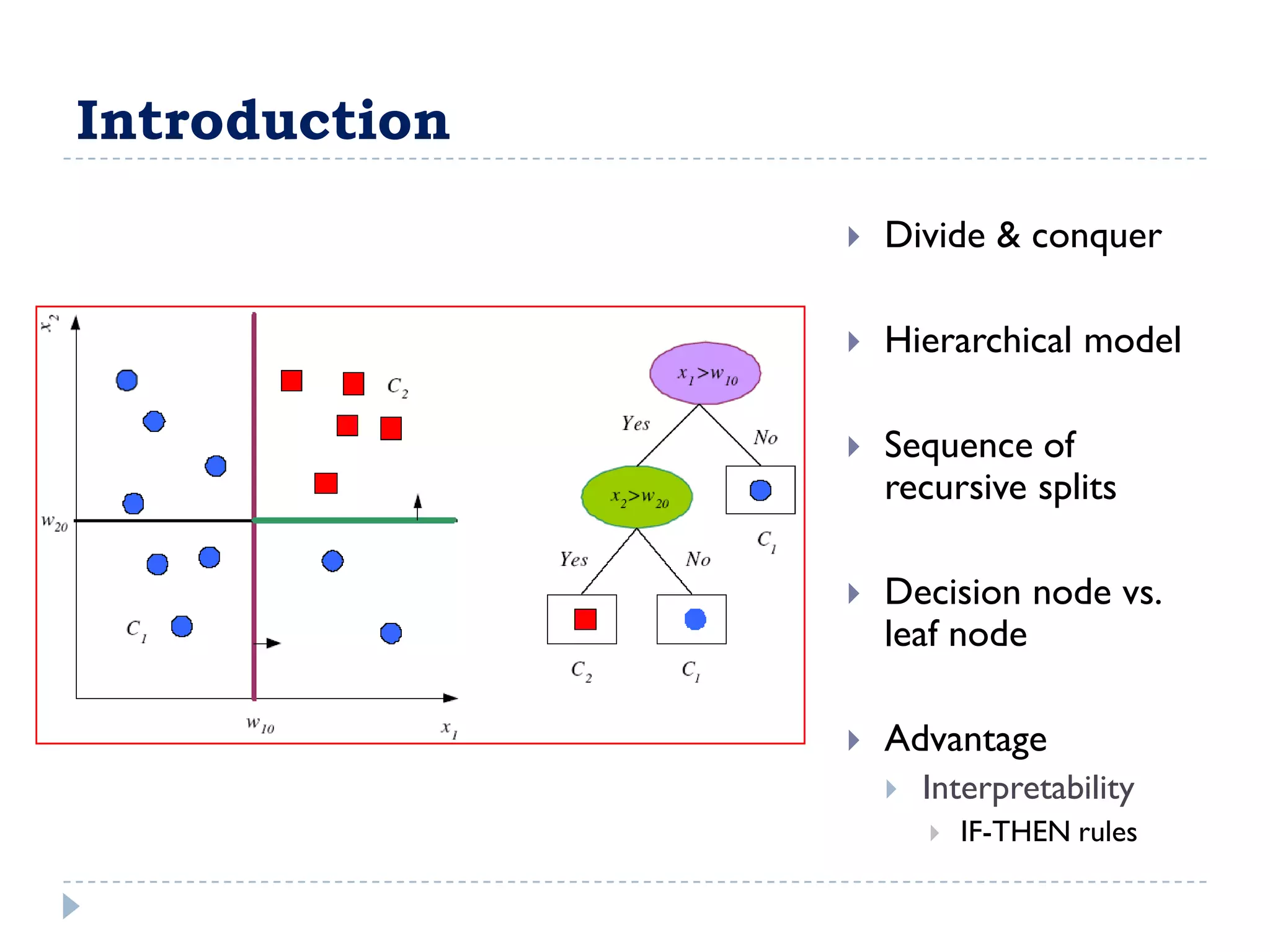
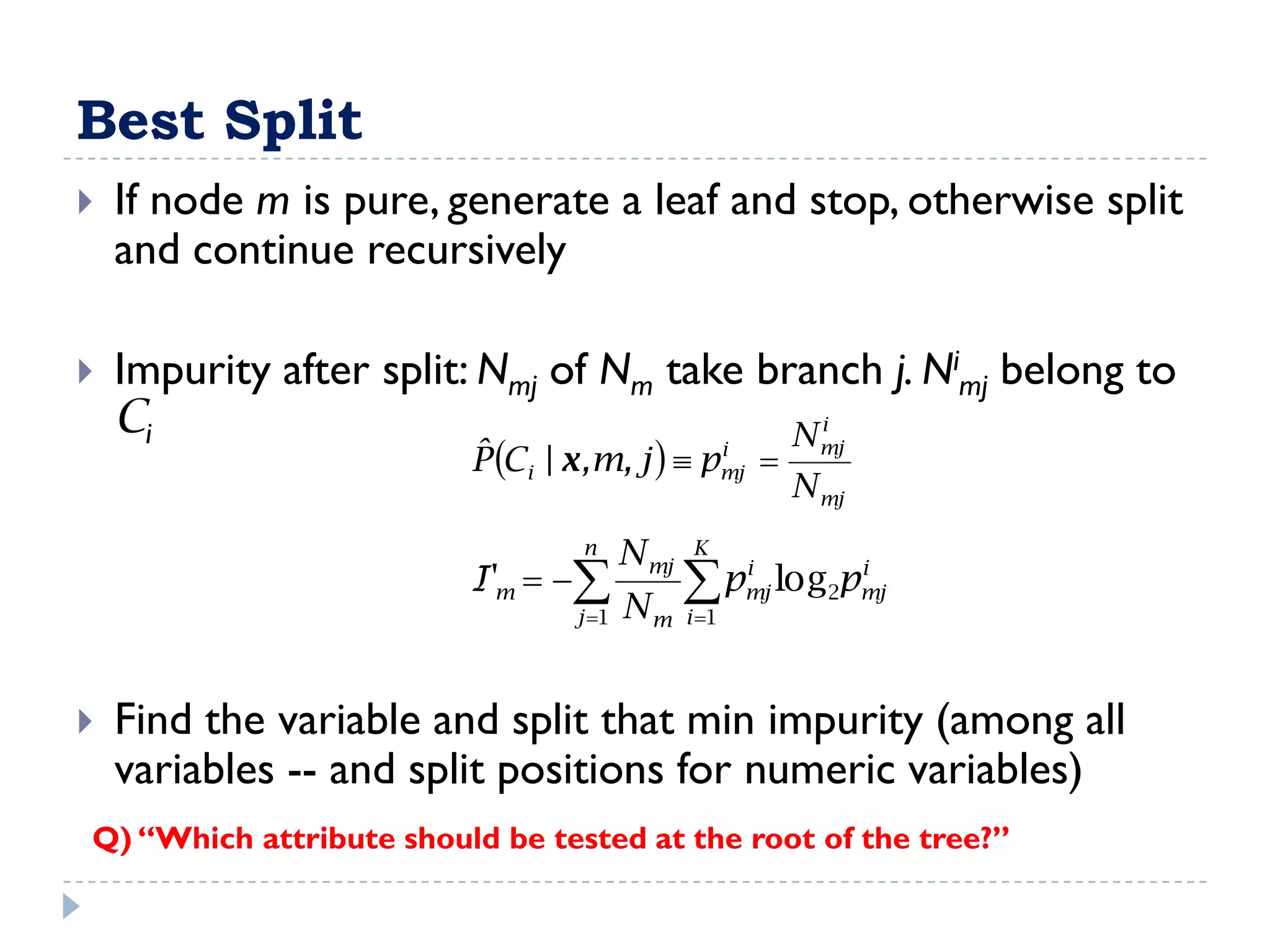
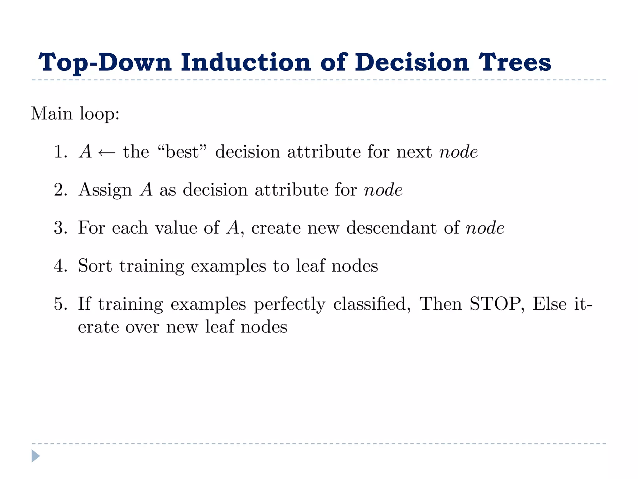
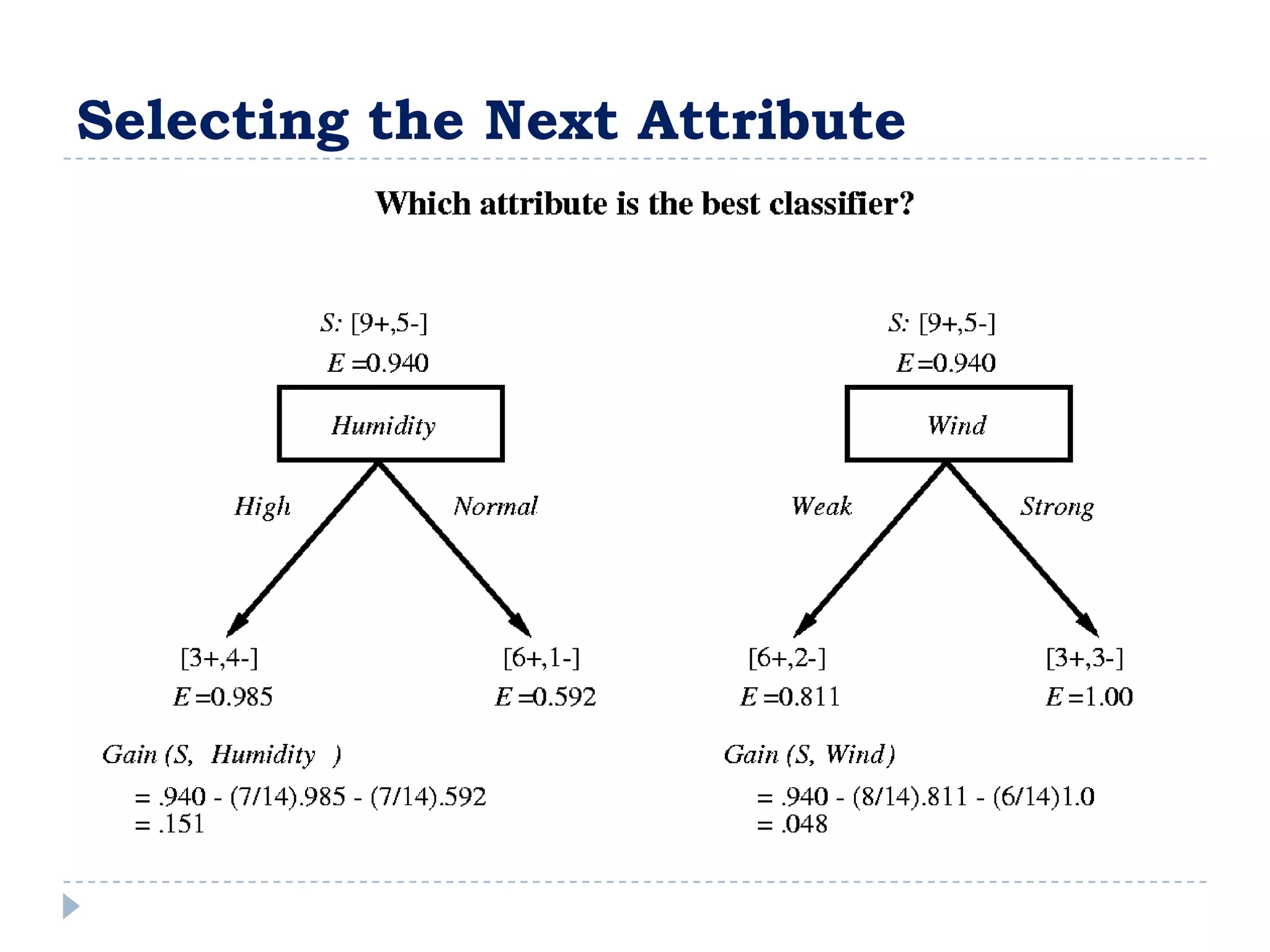
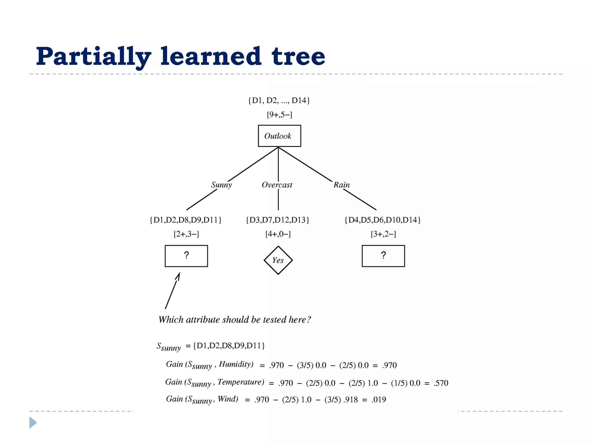
The attribute that should be tested at the root of the decision tree is the attribute that results in the maximum information gain, or minimum entropy, when used to split the training data. In other words, the attribute that best separates the data according to the target classes. This attribute will create "purer" nodes with respect to the target classes.

1. Introduction to Machine Learning
Jinhyuk Choi
Human-Computer Interaction Lab @ Information and Communications University

2. Contents
 Concepts of Machine Learning
 Multilayer Perceptrons
 Decision Trees
 Bayesian Networks

3. What is Machine Learning?
 Large storage / large amount of data
 Looks random but certain patterns
 Web log data
 Medical record
 Network optimization
 Bioinformatics
 Machine vision
 Speech recognition…
 No complete identification of the process
 A good or useful approximation

4. What is Machine Learning?
Definition
 Programming computers to optimize a
performance criterion using example data or past
experience
 Role of Statistics
 Inference from a sample
 Role of Computer science
 Efficient algorithms to solve the optimization problem
 Representing and evaluating the model for inference
 Descriptive (training) / predictive (generalization)
Learning from Human-generated data??

5. What is Machine Learning?
Concept Learning
• Inducing general functions from specific training examples (positive or
negative)
• Looking for the hypothesis that best fits the training examples
Objects Concept
눈, 코, 다리 Bird
생식능력, 날개, 부리,
boolean function :
… 깃털… Bird(animal)  “true or not”
무생물…
• Concepts:
- describing some subset of objects or events defined over a larger set
- a boolean-valued function

6. What is Machine Learning?
Concept Learning
 Inferring a boolean-valued function from training examples of its input and
output
Hypothesis 1
Hypothesis 2
Concept
Web log data
Medical record
Network optimization
Positive examples Bioinformatics
Negative examples Machine vision
Speech recognition…

7. What is Machine Learning?
Learning Problem Design
 Do you enjoy sports ?
 Learn to predict the value of “EnjoySports” for an arbitrary day, based on
the value of its other attributes
 What problem?
 Why learning?
 Attributes selection
 Effective?
 Enough?
 What learning algorithm?

8. Applications
 Learning associations
 Classification
 Regression
 Unsupervised learning
 Reinforcement learning

9. Examples (1)
 TV program preference inference based on web usage data
Web page #1 TV Program #1
Web page #2 TV Program #2
Web page #3 Classifier TV Program #3
Web page #4 1 2 TV Program #4
…. ….
3
What are we supposed to do at each step?

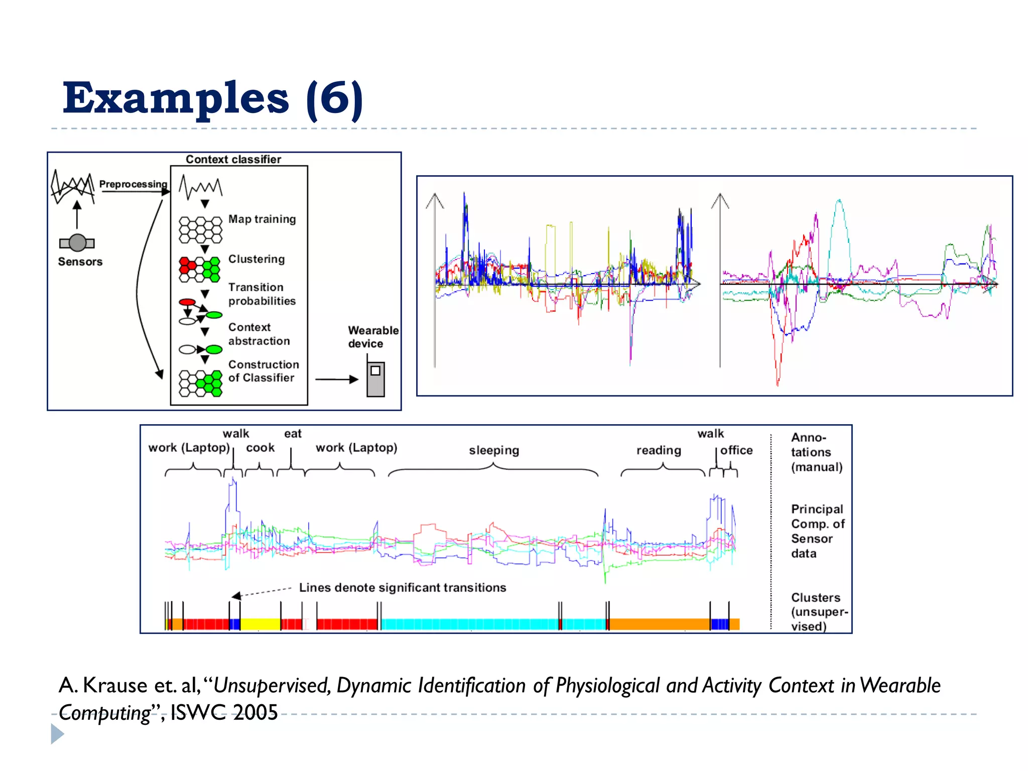
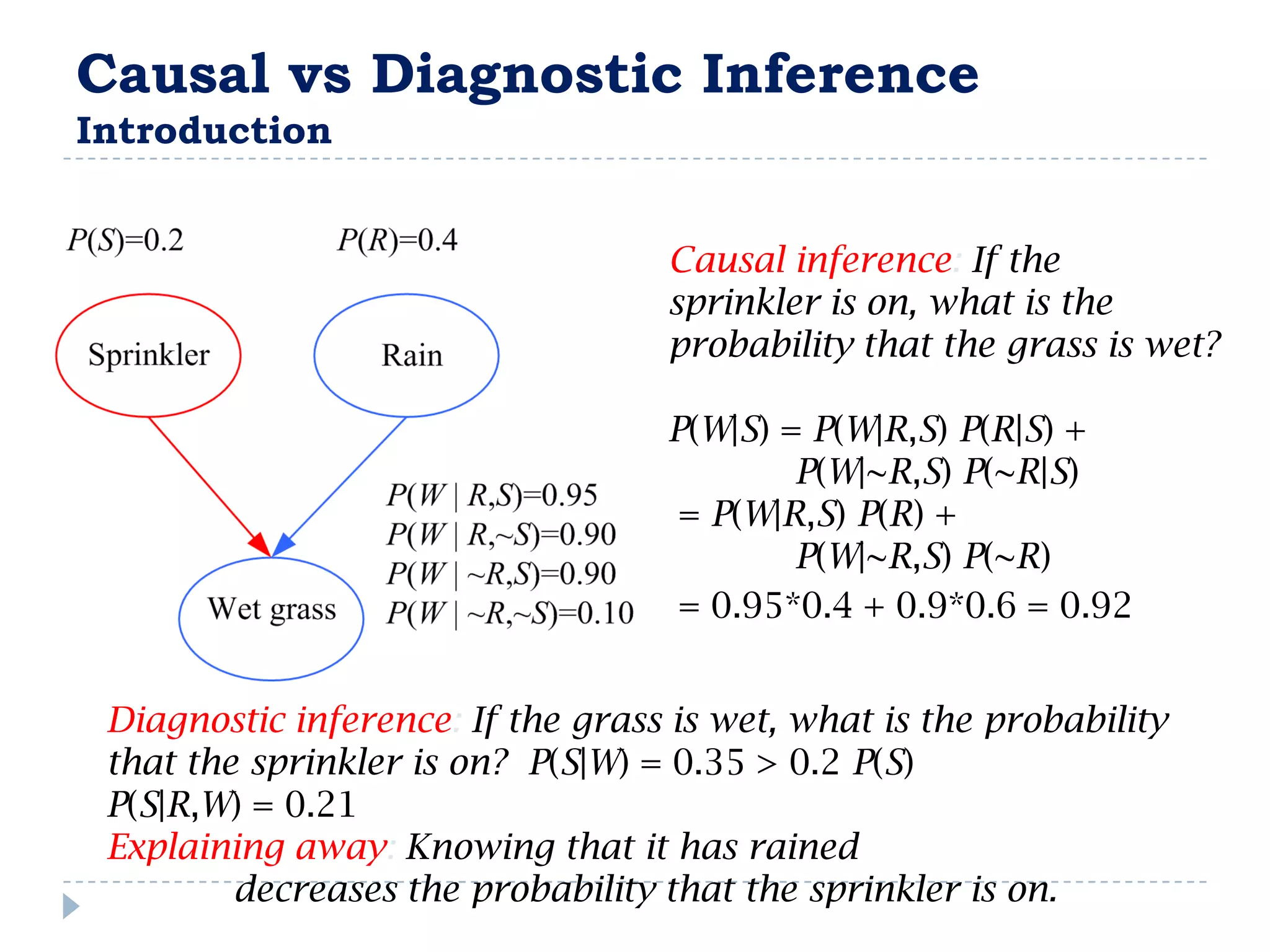
10. Examples (2)
from a HW of Neural Networks Class (KAIST-2002)
 Function approximation (Mexican hat)
 
f3 ( x1 , x2 )  sin 2 x12  x2 ,
2
x1 , x2 [1,1]

11. Examples (3)
from a HW of Machine Learning Class (ICU-2006)
 Face image classification

12. Examples (4)
from a HW of Machine Learning Class (ICU-2006)

13. Examples (5)
from a HW of Machine Learning Class (ICU-2006)
 Sensay

14. Examples (6)
A. Krause et. al, “Unsupervised, Dynamic Identification of Physiological and Activity Context in Wearable
Computing”, ISWC 2005

15. #1. Multilayer Perceptrons

16. Neural Network?
VS. Adaline
MLP
SOM
Hopfield network
RDFN
Bifurcating neuron networks
…

17. Multilayer Networks of Sigmoid Units
• Supervised learning
• 2-layer
• Fully connected
Really looks like the brain??

18. Sigmoid Unit

19. The back-propagation algorithm
 Network model
Input layer hidden layer output layer
xi yj ok
v ji
wkj
   
y j  s  v ji x i 
   w y 
ok  s  kj j 

 i
 
 
 
j 
  1
E v , w    tk  ok 
2
 Error function: 2 k
 Stochastic gradient descent

20. Gradient-Descent Function Minimization

21. Gradient-descent function minimization
 
 In order to find a vector parameter x that minimizes a function f x  …
 
 Start with a random initial value of x  x 0 .
 Determine the direction of the steepest descent in the parameter space by
 f f f  

f    , ,..., 
 x x
 1 2 x n 


 Move to the direction a step.
 
 x i  1  x i   hf 
x
 Repeat the above two steps until no more change in .
 For gradient-descent to work…
 The function to be minimized should be continuous.
 The function should not have too many local minima.

22. Back-propagation

23. Derivation of back-propagation algorithm
Adjustment of wkj :
2
E  1 2 1   t  s  w y 



   tk  ok     k
  k j j 
wk j  wk j   2 k  2 wk j   
 j
 


1
 y j ok  1  ok  1 2 tk   ok  
2
 y j ok  1  ok  tk   ok  
E
wkj  h  h ok 1  ok tk  ok y j
wkj 
o 
d k

24. Derivation of back-propagation algorithm
Adjustment of vji :
2
E  1 2 1   t  s  w y 



   tk  ok       kj j 

v j i  v j i   2 k  2 k v j i   k



 j
 

2
1   t  s  w s  v x 
 
  k
  kj  ji i 
  
2 k v j i    j
  i
 

1
  x i y j  1  y j   wkj ok 1  ok 1 2 tk  ok 
2 k
 x i y j  1  y j    wkj ok 1  ok tk  ok 
k
E
v ji  h  hy j 1  y j   wkjok 1  ok tk  ok x i
v ji k
 h y j 1  y j   wkj dko x i

y k 
dj

25. Backpropagation

26. Batch learning vs. Incremental learning
Batch standard backprop proceeds as
Incremental standard backprop can be done as follows:
follows:
Initialize the weights W.
Initialize the weights W.
Repeat the following steps for j = 1 to NL:
Repeat the following steps:
Process one training case (y_j,X_j) to compute the gradient
Process all the training data DL to compute the gradient
of the error (loss) function Q(y_j,X_j,W).
of the average error function AQ(DL,W).
Update the weights by subtracting the gradient times the
Update the weights by subtracting the gradient times the
learning rate.
learning rate.

27. Training

28. Overfitting

29. #2. Decision Trees

30. Introduction
 Divide & conquer
 Hierarchical model
 Sequence of
recursive splits
 Decision node vs.
leaf node
 Advantage
 Interpretability
 IF-THEN rules

31. Divide and Conquer
 Internal decision nodes
 Univariate: Uses a single attribute, xi
 Numeric xi : Binary split : xi > wm
 Discrete xi : n-way split for n possible values
 Multivariate: Uses all attributes, x
 Leaves
 Classification: Class labels, or proportions
 Regression: Numeric; r average, or local fit
 Learning
 Construction of the tree using training examples
 Looking for the simplest tree among the trees that code the training
data without error
 Based on heuristics
 NP-complete
 “Greedy”; find the best split recursively (Breiman et al, 1984; Quinlan, 1986, 1993)

32. Classification Trees
 Split is main procedure for tree
construction
 By impurity measure
 For node m, Nm instances reach m, Nim
belong to Ci
i
ˆ Ci | x ,m  pm 
i Nm
P
Nm To be pure!!!
 Node m is pure if pim is 0 or 1
K
 Measure of impurity is entropy Im   pm log2pm
i i
i 1

33. Representation
 Each node specifies a test of some attribute of the instance
 Each branch correspond to one of the possible values for this
attribute

34. Best Split
 If node m is pure, generate a leaf and stop, otherwise split
and continue recursively
 Impurity after split: Nmj of Nm take branch j. Nimj belong to
Ci i
N mj
ˆ Ci | x ,m, j   pmj 
P i
N mj
n N mj K
I'm   p i
mj
i
log2pmj
j 1 Nm i 1
 Find the variable and split that min impurity (among all
variables -- and split positions for numeric variables)
Q) “Which attribute should be tested at the root of the tree?”

35. Top-Down Induction of Decision Trees

36. Entropy
 “Measure of uncertainty”
 “Expected number of bits to resolve uncertainty”
 Suppose Pr{X = 0} = 1/8
 If other events are equally likely, the number of events is 8. To indicate
one out of so many events, one needs lg 8 bits.
 Consider a binary random variable X s.t. Pr{X = 0} = 0.1.
 1  0.1 lg
1 1
 The expected number of bits: 0.1 lg
0.1 1  0.1
 In general, if a random variable X has c values with prob. p_c:
c c
1
 The expected number of bits: H   pi lg   pi lg pi
i 1 pi i 1

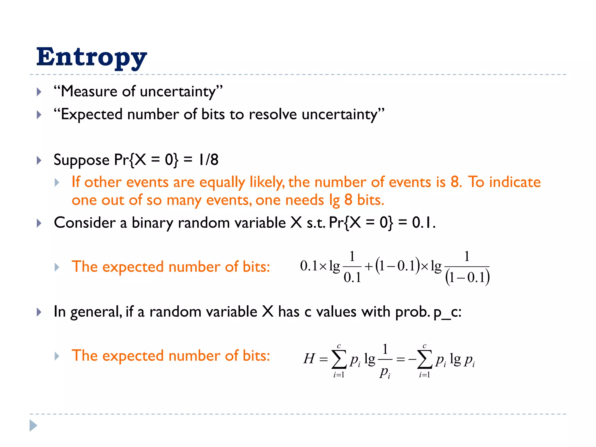
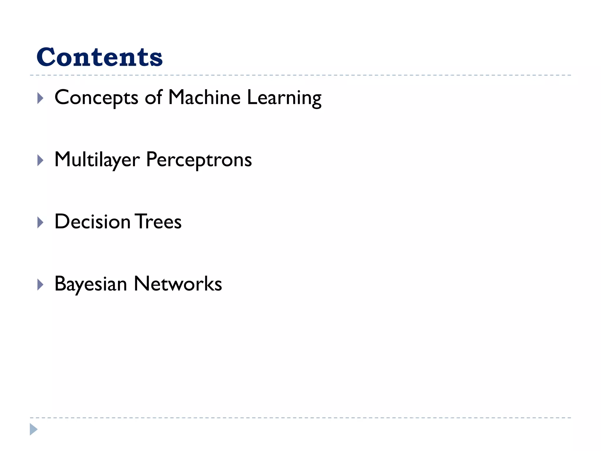
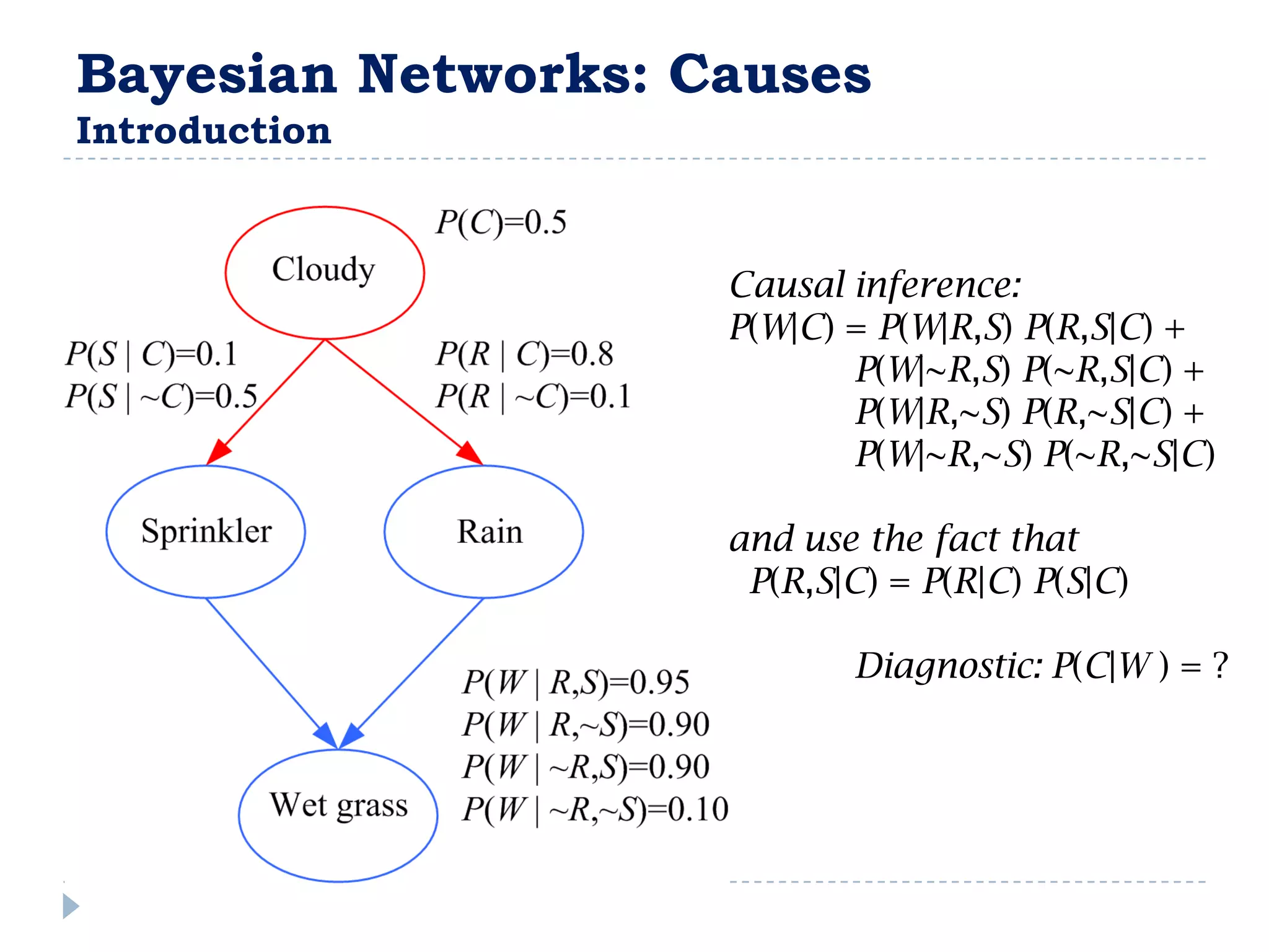
37. Entropy
Example
 14 examples
Entropy([9,5])
 (9 /14) log 2 (9 /14)  (5 /14) log 2 (5 /14)  0.940
Entropy 0 : all members positive or negative
Entropy 1 : equal number of positive & negative
0 < Entropy < 1 : unequal number of positive & negative

38. Information Gain
 Measures the expected reduction in entropy caused by partitioning
the examples

39. Information Gain
• # of samples = 100
ICU-Student tree • # of positive samples = 50
Candidate • Entropy = 1
Left side:
• # of samples = 50
Gender • # of positive samples = 40
• Entropy = 0.72
Right side:
Male Female • # of samples = 50
• # of positive samples = 10
• Entropy = 0.72
IQ Height On average
• Entropy = 0.5 * 0.72 + 0.5*0.72
= 0.72
• Reduction in entropy = 0.28
 Information gain

40. Training Examples

41. Selecting the Next Attribute

42. Partially learned tree

43. Hypothesis Space Search
 Hypothesis space: the set of
all possible decision trees
 DT is guided by information
gain measure.
Occam’s razor ??

44. Overfitting
• Why “over”-fitting?
– A model can become more complex than the true target
function(concept) when it tries to satisfy noisy data as well

45. Avoiding over-fitting the data
 Two classes of approaches to avoid overfitting
 Stop growing the tree earlier.
 Post-prune the tree after overfitting
 Ok, but how to determine the optimal size of a tree?
 Use validation examples to evaluate the effect of pruning (stopping)
 Use a statistical test to estimate the effect of pruning (stopping)
 Use a measure of complexity for encoding decision tree.
 Approaches based on the first strategy
 Reduced error pruning
 Rule post-pruning

46. Rule Extraction from Trees
C4.5Rules
(Quinlan, 1993)

47. #3. Bayesian Networks

48. Bayes’ Rule
Introduction
prior likelihood
posterior
P C  p x | C 
P C | x  
p x 
evidence
P C  0  P C  1  1
p x   p x | C  1P C  1  p x | C  0P C  0
p C  0 | x   P C  1 | x   1

49. Bayes’ Rule: K>2 Classes
Introduction
p x | Ci P Ci 
P Ci | x  
p x 
p x | Ci P Ci 
 K
 p x | Ck P Ck 
k 1
K
P Ci   0 and  P Ci   1
i 1
choose Ci if P Ci | x   max k P Ck | x 

50. Bayesian Networks
Introduction
 Graphical models, probabilistic networks
 causality and influence
 Nodes are hypotheses (random vars) and the prob corresponds to our
belief in the truth of the hypothesis
 Arcs are direct influences between hypotheses
 The structure is represented as a directed acyclic graph (DAG)
 Representation of the dependencies among random variables
 The parameters are the conditional probs in the arcs
Small set of all possible
probability, relating B.N. combinations of
only neighbor node cicumstances

51. Bayesian Networks
Introduction
 Learning
 Inducing a graph
 From prior knowledge
 From structure learning
 Estimating parameters
 EM
 Inference
 Beliefs from evidences
 Especially among the nodes not directly connected

52. Structure
Introduction
 Initial configuration of BN
 Root nodes
 Prior probabilities
 Non-root nodes
 Conditional probabilities given all possible combinations of direct
predecessors
P(a) P(b)
A B
P(c|a)
C D P(d|ab), P(d|aㄱb), P(d|ㄱab), P(d|ㄱaㄱb)
P(c|ㄱa)
P(e|d) E
P(e|ㄱd)

53. Causes and Bayes’ Rule
Introduction
Diagnostic inference:
diagnostic Knowing that the grass is wet,
what is the probability that rain is
causal the cause?
P W | R P R 
P R | W  
P W 
P W | R P R 

P W | R P R   P W |~ R P ~ R 
0.9  0.4
  0.75
0.9  0.4  0.2  0.6

54. Causal vs Diagnostic Inference
Introduction
Causal inference: If the
sprinkler is on, what is the
probability that the grass is wet?
P(W|S) = P(W|R,S) P(R|S) +
P(W|~R,S) P(~R|S)
= P(W|R,S) P(R) +
P(W|~R,S) P(~R)
= 0.95*0.4 + 0.9*0.6 = 0.92
Diagnostic inference: If the grass is wet, what is the probability
that the sprinkler is on? P(S|W) = 0.35 > 0.2 P(S)
P(S|R,W) = 0.21
Explaining away: Knowing that it has rained
decreases the probability that the sprinkler is on.

55. Bayesian Networks: Causes
Introduction
Causal inference:
P(W|C) = P(W|R,S) P(R,S|C) +
P(W|~R,S) P(~R,S|C) +
P(W|R,~S) P(R,~S|C) +
P(W|~R,~S) P(~R,~S|C)
and use the fact that
P(R,S|C) = P(R|C) P(S|C)
Diagnostic: P(C|W ) = ?

56. Bayesian Nets: Local structure
Introduction
P (F | C) = ?
d
P X 1 , X d    P X i | parentsX i 
i 1

57. Bayesian Networks: Inference
Introduction
 P (C,S,R,W,F ) = P (C ) P (S |C ) P (R |C ) P (W |R,S ) P (F |R )
 P (C,F ) = ∑S ∑R ∑W P (C,S,R,W,F )
 P (F |C) = P (C,F ) / P(C ) Not efficient!
 Belief propagation (Pearl, 1988)
 Junction trees (Lauritzen and Spiegelhalter, 1988)
 Independence assumption

58. Inference
Evidence & Belief Propagation
 Evidence – values of observed nodes
 V3 = T,V6 = 3 V1
 Our belief in what the value of Vi
„should‟ be changes.
 This belief is propagated V3 V2
 As if the CPTs became
V4
V3=T 1.0 P V2=T V2=F
V3=F 0.0 V6=1 0.0 0.0
V5 V6
V6=2 0.0 0.0
V6=3 1.0 1.0

59. Belief Propagation
Bayes Law:
P( B | A) P( A)
P( A | B) 
P( B)
“Causal” message “Diagnostic” message
Going down arrow, sum out parent Going up arrow, Bayes Law
Message
Messages
Specifically:
1/a
9
* some figures from: Peter Lucas BN lecture course

60. The  Messages
• What are the messages?
• For simplicity, let the nodes be binary
V1=T 0.8 The message passes on information.
V1=F 0.2 What information? Observe:
V1
P(V2| V1) = P(V2| V1=T)P(V1=T)
+ P(V2| V1=F)P(V1=F)
P V1=T V1=F The information needed is the CPT
of V1 = V(V1)
V2 V2=T 0.4 0.9
V2=F 0.6 0.1  Messages capture information
passed from parent to child

61. The  Messages
• We know what the  messages are
• What about ?
Assume E = { V2 } and compute by Bayes‟rule:
V1 P(V1 ) P(V2 | V1 )
P(V1 | V2 )   aP(V1 ) P(V2 | V1 )
P(V2 )
The information not available at V1 is the P(V2|V1). To be
V2 passed upwards by a -message. Again, this is not in general
exactly the CPT, but the belief based on evidence down the tree.

62. Belief Propagation
U1 U2
λ(U2)
π(U1)
π(U2)
λ(U1)
V
λ(V1)
π(V2)
π(V1)
λ(V2)
V1 V2

63. Evidence & Belief
V1 Evidence
Belief V3 V2
V4
V5 V6
Evidence
Works for classification ??

64. Naive Bayes’ Classifier
Given C, xj are independent:
p(x|C) = p(x1|C) p(x2|C) ... p(xd|C)

65. Application Procedures
For classification
 MLP
 Data collection & Pre-processing (Training data / Test data)
 Decision node selection (output node)
 Network training
 Generalization
 Parameter tuning & Pruning
 Final network
 Decision Trees
 Data collection & Pre-processing (Training data / Test data)
 Decision attribute selection
 Tree construction
 Pruning
 Final tree
 Bayesian Networks
 Data collection & Pre-processing (Training data / Test data)
 Structure configuration
 Prior knowledge
 Parameter learning
 Decision node selection
 Inference (classification)
 Evidence & belief
 Final network

66. Simulation
 Simulation Packages
 WEKA (JAVA)
 http://www.cs.waikato.ac.nz/ml/weka/
 FullBNT (MATLAB)
 http://www.cs.ubc.ca/~murphyk/Software/BNT/bnt.html
 MSBNx
 http://research.microsoft.com/msbn/
 MATLAB Neural Networks Toolbox
 http://www.mathworks.com/products/neuralnet/
 C4.5
 http://www.rulequest.com/Personal/

67. WEKA

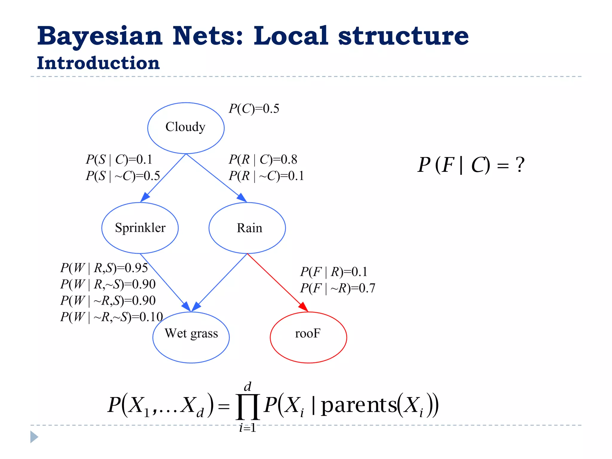
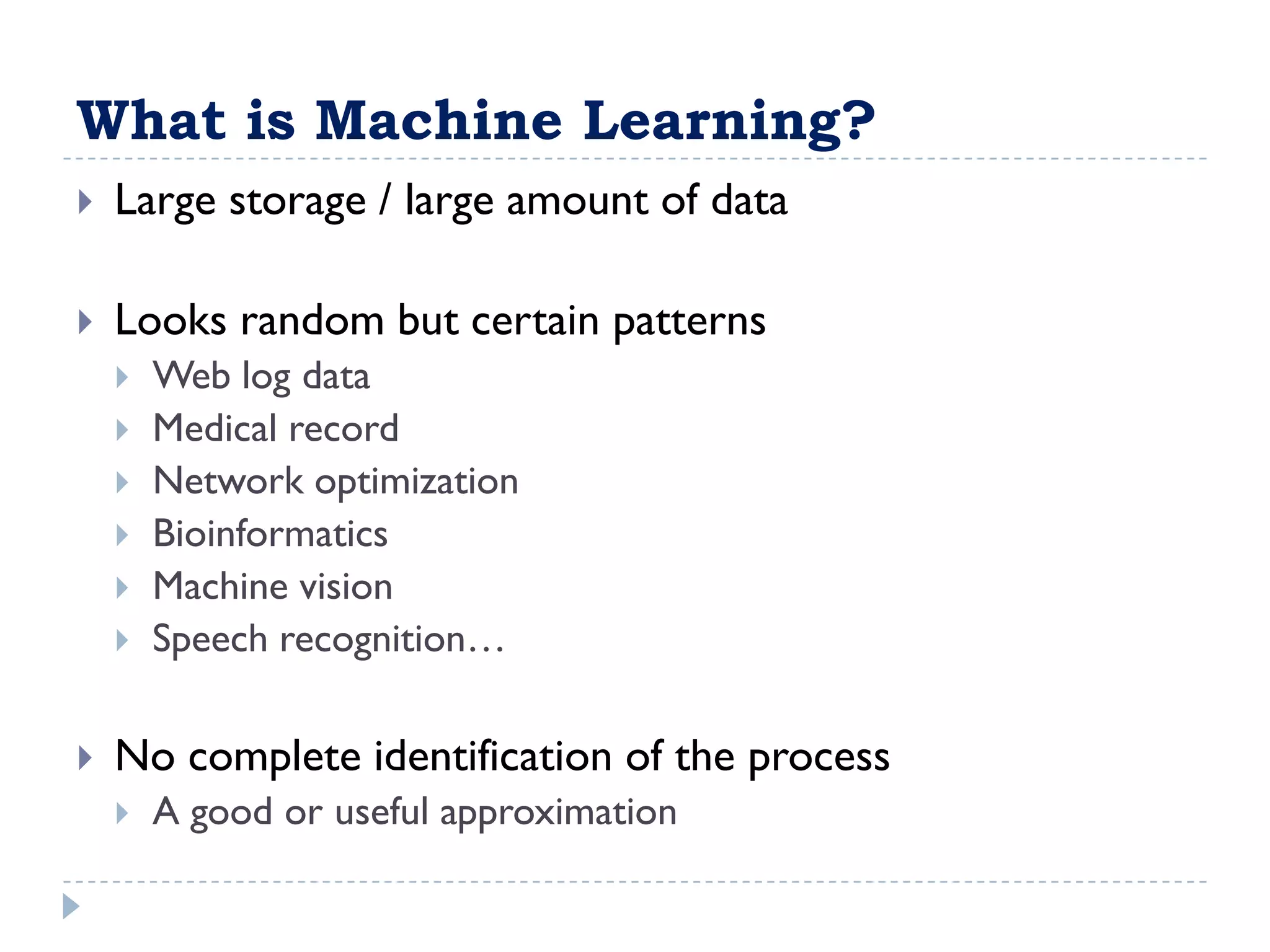
68. FullBNT
 clear all
 N = 4; % 노드의 개수
 dag = zeros(N,N); % 네크워크 구조 shell
 C = 1; S = 2; R = 3; W = 4; % 각 노드 Naming
 dag(C,[R S]) = 1; % 네트워크 구조 명시
 dag(R,W) = 1;
 dag(S,W)=1;
 %discrete_nodes = 1:N;
 node_sizes = 2*ones(1,N); % 각 노드가 가질 수 있는 값의 개수
 %node_sizes = [4 2 3 5];
 %onodes = [];
 %bnet = mk_bnet(dag, node_sizes, 'discrete', discrete_nodes, 'observed', onodes);
 bnet = mk_bnet(dag, node_sizes, 'names', {'C','S','R','W'}, 'discrete', 1:4);
 %C = bnet.names('cloudy'); % bnet.names is an associative array
 %bnet.CPD{C} = tabular_CPD(bnet, C, [0.5 0.5]);
 %%%%%% Specified Parameters
 %bnet.CPD{C} = tabular_CPD(bnet, C, [0.5 0.5]);
 %bnet.CPD{R} = tabular_CPD(bnet, R, [0.8 0.2 0.2 0.8]);
 %bnet.CPD{S} = tabular_CPD(bnet, S, [0.5 0.9 0.5 0.1]);
 %bnet.CPD{W} = tabular_CPD(bnet, W, [1 0.1 0.1 0.01 0 0.9 0.9 0.99]);

69. MSBNx

70. References
 Textbooks
 Ethem ALPAYDIN, Introduction to Machine Learning, The MIT Press, 2004
 Tom Mitchell, Machine Learning, McGraw Hill, 1997
 Neapolitan, R.E., Learning Bayesian Networks, Prentice Hall, 2003
 Materials
 Serafí Moral, Learning Bayesian Networks, University of Granada, Spain
n
 Zheng Rong Yang, Connectionism, Exeter University
 KyuTae Cho ,Jeong Ki Yoo ,HeeJin Lee, Uncertainty in AI, Probabilistic reasoning,
Especially for Bayesian Networks
 Gary Bradski, Sebastian Thrun, Bayesian Networks in Computer Vision, Stanford
University
 Recommended Textbooks
 Christopher M. Bishop, Pattern Recognition and Machine Learning, Springer, 2006
 J. Ross Quinlan, C4.5: Programs for Machine Learning, Morgan Kaufmann, 1992
 Haykin, Simon S., Neural networks : a comprehensive foundation, Prentice Hall, 1999
 Jensen, Finn V., Bayesian networks and decision graphs, Springer, 2007