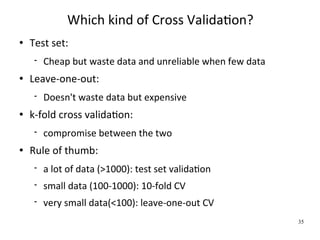
This document provides an introduction to machine learning. It defines machine learning as developing algorithms that allow computers to learn from experience to improve their performance on tasks. The document outlines supervised learning and other learning frameworks. It discusses applications of machine learning such as autonomous vehicles, recommendation systems, and credit risk analysis. The document also provides examples of machine learning applications at the University of Liege including medical diagnosis, gene expression analysis, and patient classification.

1. An introducWon to
Machine Learning
Pierre Geurts
p.geurts@ulg.ac.be
Department of EE and CS &
GIGA‐R, BioinformaWcs and modelling
University of Liège

2. Outline
● IntroducWon
● Supervised Learning
● Other learning protocols/frameworks
2

3. Machine Learning: definiWon
 Machine Learning is concerned with the development,
the analysis, and the application of algorithms that
allow computers to learn
 Learning:
 A computer learns if it improves its performance at some
task with experience (i.e. by collecWng data)
 ExtracWng a model of a system from the sole observaWon (or
the simulaWon) of this system in some situaWons.
 A model = any relaWonship between the variables used to
describe the system.
 Two main goals: make predicWon and beXer understand the
system
3

4. Machine learning: when ?
 Learning is useful when:
 Human expertise does not exist
navigating on Mars
 Humans are unable to explain their expertise
speech recognition
 Solution changes in time
routing on a computer network
 Solution needs to be adapted to particular cases
user biometrics
 Example:
 It is easier to write a program that learns to play checkers or
backgammon well by self-play rather than converting the 4
expertise of a master player to a program.

5. ApplicaWons: autonomous driving
 DARPA Grand challenge 2005: build a robot capable of
navigaWng 240 km through desert terrain in less than 10
hours, with no human intervenWon
 The actual wining Wme of Stanley [Thrun et al., 05] was 6
hours 54 minutes.
http://www.darpa.mil/grandchallenge/ 5

6. ApplicaWons: recommendaWon system
 NeVlix prize: predict how much someone is going to love a
movie based on their movies preferences
 Data: over 100 million raWngs that over 480,000 users gave to
nearly 18,000 movies
 Reward: $1,000,000 dollars if 10% improvement with respect to
NeVlix's current system (two teams succeed this summer)
http://www.netflixprize.com 6

7. ApplicaWons: credit risk analysis
 Data:
 Logical rules automaWcally learned from data:
7

8. Other applicaWons
 Machine learning has a wide spectrum of applicaWons
including:
 Retail: Market basket analysis, Customer relaWonship
management (CRM)
 Finance: Credit scoring, fraud detecWon
 Manufacturing: OpWmizaWon, troubleshooWng
 Medicine: Medical diagnosis
 TelecommunicaWons: Quality of service opWmizaWon, rouWng
 BioinformaWcs: MoWfs, alignment
 Web mining: Search engines
 ...
8

9. Some applicaWons at ULG (1/4)
9

10. Some applicaWons at ULG (2/4)
10

11. Some applicaWons at ULG (3/4)
11

12. Some applicaWons at ULG (4/4)
12

13. Related fields
 ArWficial Intelligence: smart algorithms
 StaWsWcs: inference from a sample
 Computer Science: efficient algorithms and complex
models
 Systems and control: analysis, modeling, and control of
dynamical systems
 Data Mining: searching through large volumes of data
13

14. Problem definition
One part of the data
Data generation mining process
Raw data
 Each step generates many quesWons:
 Data generaWon: data types, sample
Preprocessing size, online/offline...
 Preprocessing: normalizaWon, missing
Preprocessed data values, feature selecWon/extracWon...
 Machine learning: hypothesis, choice of
learning paradigm/algorithm...
Machine
learning  Hypothesis validaWon: cross‐validaWon,
model deployment...
Hypothesis
Validation
Knowledge/Predictive model
14

15. Glossary
 Data=a table (dataset, database, sample)
Variables (attributes, features) =
measurements made on objects
VAR 1 VAR 2 VAR 3 VAR 4 VAR 5 VAR 6 VAR 7 VAR 8 VAR 9 VAR 10 VAR 11 ...
Object 1 0 1 2 0 1 1 2 1 0 2 0 ...
Object 2 2 1 2 0 1 1 0 2 1 0 2 ...
Object 3 0 0 1 0 1 1 2 0 2 1 2 ...
Object 4 1 1 2 2 0 0 0 1 2 1 1 ...
Object 5 0 1 0 2 1 0 2 1 1 0 1 ...
Object 6 0 1 2 1 1 1 1 1 1 1 1 ...
Object 7 2 1 0 1 1 2 2 2 1 1 1 ...
Object 8 2 2 1 0 0 0 1 1 1 1 2 ...
Object 9 1 1 0 1 0 0 0 0 1 2 1 ...
Object 10 1 2 2 0 1 0 1 2 1 0 1 ...
... ... ... ... ... ... ... ... ... ... ... ... ...
Objects (samples, observations,
individuals, examples, patterns) Dimension=number of variables
Size=number of objects
 Objects: samples, paWents, documents, images...
 Variables: genes, proteins, words, pixels...
15

16. Outline
● IntroducWon
● Supervised Learning
 IntroducWon
 Model selecWon, cross‐validaWon, overfiYng
 Some supervised learning algorithms
 Beyond classificaWon and regression
● Other learning protocols/frameworks
16

17. Supervised learning
Inputs Output
X1 X2 X3 X4 Y Supervised
-0.61 -0.43 Y 0.51 Healthy learning
-2.3 -1.2 N -0.21 Disease
0.33 -0.16 N 0.3 Healthy
0.23 -0.87 Y 0.09 Disease
-0.69 0.65 N 0.58 Healthy
0.61 0.92 Y 0.02 Disease
model,
Learning sample hypothesis
 Goal: from the database (learning sample), find a funcWon f of the
inputs that approximates at best the output
 Formally:
17
 Symbolic output ⇒ classificaEon, Numerical output ⇒ regression

18. Two main goals
 PredicWve:
Make predictions for a new sample described by its
attributes
X1 X2 X3 X4 Y
-0.71 -0.27 T -0.72 Healthy
-2.3 -1.2 F -0.92 Disease
0.42 0.26 F -0.06 Healthy
0.84 -0.78 T -0.3 Disease
-0.55 -0.63 F -0.02 Healthy
0.07 0.24 T 0.4 Disease
0.75 0.49 F -0.88 ?
 InformaWve:
Help to understand the relationship between the inputs
and the output
Find the most relevant inputs
18

19. Example of applicaWons
 Biomedical domain: medical diagnosis, differenWaWon of
diseases, predicWon of the response to a treatment...
Gene expression, Metabolite concentrations...
X1 X2 ... X4 Y
-0.1 0.02 ... 0.01 Healthy
-2.3 -1.2 ... 0.88 Disease
Patients 0 0.65 ... -0.69 Healthy
0.71 0.85 ... -0.03 Disease
-0.18 0.14 ... 0.84 Healthy
-0.64 0.15 ... 0.03 Disease
19

20. Example of applicaWons
 Perceptual tasks: handwriXen character recogniWon,
speech recogniWon...
 Inputs:
● a grey intensity [0,255] for
each pixel
● each image is
represented by a vector of
pixel intensities
● eg.: 32x32=1024
dimensions
 Output:
● 9 discrete values
● Y={0,1,2,...,9}
20

21. Example of applicaWons
 Time series predicWon: predicWng electricity load, network
usage, stock market prices...
21

22. Outline
● IntroducWon
● Supervised Learning
 IntroducWon
 Model selecWon, cross‐validaWon, overfiYng
 Some supervised learning algorithms
 Beyond classificaWon and regression
● Other learning protocols/frameworks
22

23. IllustraWve problem
 Medical diagnosis from two measurements (eg., weights and
temperature)
1
X1 X2 Y
0.93 0.9 Healthy
0.44 0.85 Disease
0.53 0.31 Healthy
X2
0.19 0.28 Disease
... ... ...
0.57 0.09 Disease
0.12 0.47 Healthy
0
0 1
X1
 Goal: find a model that classifies at best new cases for which
X1 and X2 are known
23

24. Learning algorithm
 A learning algorithm is defined by:
 a family of candidate models (=hypothesis space H)
 a quality measure for a model
 an opWmizaWon strategy
 It takes as input a learning sample and outputs a funcWon h
in H of maximum quality
1
a model
obtained by
supervised
X2
learning
0
0 1
X1
24

25. Linear model
Disease if w0+w1*X1+w2*X2>0
h(X1,X2)=
Normal otherwise
1
X2
0
0 1
X1
 Learning phase: from the learning sample, find the best
values for w0, w1 and w2
 Many alternaWves even for this simple model (LDA,
Perceptron, SVM...)
25

26. QuadraWc model
Disease if w0+w1*X1+w2*X2+w3*X12+w4*X22>0
h(X1,X2)=
Normal otherwise
1
X2
0
0 1
X1
 Learning phase: from the learning sample, find the best
values for w0, w1,w2, w3 and w4
 Many alternaWves even for this simple model (LDA,
Perceptron, SVM...) 26

27. ArWficial neural network
Disease if some very complex function of X1,X2>0
h(X1,X2)=
Normal otherwise
1
X2
0
0 1
X1
 Learning phase: from the learning sample, find the
numerous parameters of the very complex funcWon
27

28. Which model is the best?
linear quadratic neural net
1 1 1
0 0 0
0 1 0 1 0 1
 Why not choose the model that minimises the error rate on
the learning sample? (also called re‐subsEtuEon error)
 How well are you going to predict future data drawn from
the same distribuWon? (generalisaEon error)
28

29. The test set method
1. Randomly choose 30% of the data to
1
be in a test sample
2. The remainder is a learning sample
3. Learn the model from the learning
sample
0
4. EsWmate its future performance on
0 1
the test sample
29

30. Which model is the best?
linear quadratic neural net
1 1 1
0 0 0
0 1 0 1 0 1
LS error= 3.4% LS error= 1.0% LS error= 0%
TS error= 3.5% TS error= 1.5% TS error= 3.5%
 We say that the neural network overfits the data
 OverfiYng occurs when the learning algorithm starts fiYng
noise.
 (by opposiWon, the linear model underfits the data)
30

31. The test set method
 Upside:
 very simple
 ComputaWonally efficient
 Downside:
 Wastes data: we get an esWmate of the best method to apply
to 30% less data
 Very unstable when the database is small (the test sample
choice might just be lucky or unlucky)
31

32. Leave‐one‐out Cross ValidaWon
For k=1 to N
 remove the kth object from the
1 learning sample
 learn the model on the remaining
objects
0
 apply the model to get a predicWon
0 1 for the kth object
report the proporWon of misclassified
objects
32

33. Leave‐one‐out Cross ValidaWon
 Upside:
 Does not waste the data (you get an esWmate of the best
method to apply to N‐1 data)
 Downside:
 Expensive (need to train N models)
 High variance
33

34. k‐fold Cross ValidaWon
 Randomly parWWon the dataset into k subsets (for example 10)
TS
 For each subset:
 learn the model on the objects that are not in the subset
 compute the error rate on the points in the subset
 Report the mean error rate over the k subsets
 When k=the number of objects ⇒ leave‐one‐out cross validaWon
34

35. Which kind of Cross ValidaWon?
 Test set:
 Cheap but waste data and unreliable when few data
 Leave‐one‐out:
 Doesn't waste data but expensive
 k‐fold cross validaWon:
 compromise between the two
 Rule of thumb:
 a lot of data (>1000): test set validaWon
 small data (100‐1000): 10‐fold CV
 very small data(<100): leave‐one‐out CV
35

36. CV‐based complexity control
Error
Under-fitting Over-fitting
CV error
LS error
Optimal complexity Complexity
36

37. Complexity
 Controlling complexity is called regularizaWon or smoothing
 Complexity can be controlled in several ways
 The size of the hypothesis space: number of candidate
models, range of the parameters...
 The performance criterion: learning set performance versus
parameter range, eg. minimizes
Err(LS)+λ C(model)
 The opWmizaWon algorithms: number of iteraWons, nature of
the opWmizaWon problem (one global opWmum versus
several local opWma)...
37

38. CV‐based algorithm choice
 Step 1: compute 10‐fold (or test set or LOO) CV error for
different algorithms
Algo 4
Algo 2
CV Algo 1 Algo 3
error
 Step 2: whichever algorithm gave best CV score: learn a
new model with all data, and that's the predicWve model
 What is the expected error rate of this model?
38

39. Warning: Intensive use of CV can overfit
 If you compare many (complex) models, the probability
that you will find a good one by chance on your data
increases
 SoluWon:
 Hold out an addiWonal test set before starWng the
analysis (or, beXer, generate this data aFerwards)
 Use it to esWmate the performance of your final model
(For small datasets: use two stages of 10‐fold CV)
39

40. A note on performance measures
True class Model 1 Model 2
1
2
Negative
Negative
Posit ive
Negat ive
Negat ive
Negat ive
 Which of these two models is
3 Negative Posit ive Posit ive the best?
4 Negative Posit ive Negat ive
5 Negative Negat ive Negat ive
6 Negative Negat ive Negat ive  The choice of an error or
7
8
Negative
Negative
Negat ive
Negat ive
Posit ive
Negat ive quality measure is highly
9
10
Negative
Posit ive
Negat ive
Posit ive
Negat ive
Posit ive applicaWon dependent.
11 Posit ive Posit ive Negat ive
12 Posit ive Posit ive Posit ive
13 Posit ive Posit ive Posit ive
14 Posit ive Negat ive Negat ive
15 Posit ive Posit ive Negat ive
40

41. A note on performance measures
 The error rate is not the only way to assess a predicWve model
 In binary classificaWon, results can be summarized in a
conWngency table (aka confusion matrix)
Predicted class
Act ual class p n Tot al
p True Posit ive F alse Negative P
n F alse Posit ive True Negative N
 Various criterion
Error rate = (FP+FN)/(N+P) Sensitivity = TP/P (aka recall)
Accuracy = (TP+TN)/(N+P) Specificity = TN/(TN+FP)
= 1-Error rate
Precision = TP/(TP+FP) (aka PPV)
41

42. ROC and Precision/recall curves
 Each point corresponds to a parWcular choice of the decision
threshold
True Positive Rate
(Sensitivity)
Precision
False Positive Rate Recall
(1-Specificity) (Sensitivity)
42

43. Outline
 IntroducWon
 Model selecWon, cross‐validaWon, overfiYng
 Some supervised learning algorithms
 k‐NN
 Linear methods
 ArWficial neural networks
 Support vector machines
 Decision trees
 Ensemble methods
 Beyond classificaWon and regression
43

44. Comparison of learning algorithms
 Three main criteria:
 Accuracy:
 Measured by the generalizaWon error (esWmated by CV)
 Efficiency:
 CompuWng Wmes and scalability for learning and tesWng
 Interpretability:
 Comprehension brought by the model about the input‐output
relaWonship
 Unfortunately, there is usually a tradeoff between these
criteria
44

45. 1‐Nearest Neighbor (1‐NN)
(prototype based method, instance based learning, non‐parametric
method)
 One of the simplest learning algorithm:
 outputs as a predicWon the output associated to the sample
which is the closest to the test object
M1 M2 Y
1 0 .3 2 0 .8 1 He a lt h y
2 0 .1 5 0 .3 8 D ise a se
3 0 .3 9 0 .3 4 He a lt h y
4 0 .6 2 0 .1 1 D ise a se
5 0 .9 2 0 .4 3 ?
?
 2 2
d  5,1 =  0. 32−0 . 92   0 . 81−0 . 43  =0 . 71
d  5,2 =  0. 15− 0 .92   0 . 38−0 . 43  =0 . 77
2 2
d  5,3 =  0. 39−0 . 92   0 . 34− 0. 43  =0 . 71
2 2
d  5,4 =  0 .62−0 . 92   0 . 43−0 . 43  = 0 . 44
2 2
 closest=usually of minimal Euclidian distance
45

46. Obvious extension: k‐NN
?
 Find the k nearest neighbors (instead of only the first one)
with respect to Euclidian distance
 Output the most frequent class (classificaWon) or the
average outputs (regression) among the k neighbors.
46

47. Effect of k on the error
Error
Under-fitting Over-fitting
CV error
LS error
Optimal k k
47

48. Small exercise
 In this classificaWon problem with
two inputs:
 What it the resubsWtuWon error
(LS error) of 1‐NN?
 What is the LOO error of 1‐NN?
 What is the LOO error of 3‐NN?
 What is the LOO error of 22‐NN?
Andrew Moore
48

49. k‐NN
 Advantages:
 very simple
 can be adapted to any data type by changing the distance
measure
 Drawbacks:
 choosing a good distance measure is a hard problem
 very sensiWve to the presence of noisy variables
 slow for tesWng
49

50. Linear methods
 Find a model which is a linear combinaWons of the inputs
 Regression: y=w 0 w 1 x 1 w 2 x 2 ...w n w n
 y=c 1 w 0 w1 x1 ...w n x n0 c 2
ClassificaWon: if , otherwise
 Several methods exist to find coefficients w0,w1... corresponding to
different objecWve funcWons, opWmizaWon algorithms, eg.:
 Regression: least‐square regression, ridge regression, parWal least
square, support vector regression, LASSO...
50
 ClassificaWon: linear discriminant analysis, PLS‐discriminant analysis,
support vector machines...

51. Example: ridge regression
 Find w that minimizes (λ>0):
∑i  y i −w x i  ∥w∥
2 2
 From simple algebra, the soluWon is given by:
r T −1 T
w = X X  I  X y
where X is the input matrix and y is the output vector
 λ regulates complexity (and avoids problems related to the
singularity of XTX)
51

52. Example: perceptron
 Find w that minimizes:
∑i  y i −w x i 2
using gradient descent: given a training example  x , y 
  y−wT x
∀ j w j w j  x j
 Online algorithm, ie. that treats every example in turn (vs
Batch algorithm that treats all examples at once)
 Complexity is regulated by the learning rate η and the
number of iteraWons
 Can be adapted to classificaWon
52

53. Linear methods
 Advantages:
 simple
 there exist fast and scalable variants
 provide interpretable models through variable weights
(magnitude and sign)
 Drawbacks:
 oFen not as accurate as other (non‐linear) methods
53

54. Non‐linear extensions
 GeneralizaWon of linear methods:
 y=w 0 w1 1  xw 2 2  x 2 ...w n n  x
 Any linear methods can be applied (but regularizaWon
becomes more important)
 ArWficial neural networks (with a single hidden layer):

y= g ∑ W j g ∑ w i , j x i 
j i
where g is a non linear function (eg. sigmoid)
 (a non linear funcWon of a linear combinaWon of non linear
funcWons of linear combinaWons of inputs)
 Kernel methods:
 y=∑ w i i  x  ⇔ y=∑  j k  x j , x 
i j
where k  x , x ' =〈 x ,  x ' 〉 is the dot-product in the
54
feature space and j indexes training examples

55. ArWficial neural networks
 Supervised learning method iniWally inspired by the
behavior of the human brain
 Consists of the inter‐connecWon of several small units
 EssenWally numerical but can handle classificaWon and
discrete inputs with appropriate coding
 Introduced in the late 50s, very popular in the 90s
55

56. Hypothesis space: a single neuron
1 X2
X1 x w0
x w1 +
X2 x w2
+ tanh Y _
… X1
XN x wN
tanh
Y=tanh(w1*X1+w2*X2+…+wN*XN+w0) +1
-1
56

57. Hypothesis space:
MulW‐layers Perceptron
 Inter‐connecWon of several neurons (just like in the human
brain)
Hidden layer
Input layer
Output layer
 With a sufficient number of neurons and a sufficient number of
layers, a neural network can model any funcWon of the inputs.
57

58. Learning
 Choose a structure
 Tune the value of the parameters (connecWons between
neurons) so as to minimize the learning sample error.
 Non‐linear opWmizaWon by the back‐propagaWon algorithm.
In pracWce, quite slow.
 Repeat for different structures
 Select the structure that minimizes CV error
58

59. IllustraWve example
1
1 neuron
X2
0
0 1
X1
1
2 +2 neurons
X2
0
0 1
10 +10 neurons X1
1
... ...
X2
0 59
0 1
X1

60. ArWficial neural networks
 Advantages:
 Universal approximators
 May be very accurate (if the method is well used)
 Drawbacks:
 The learning phase may be very slow
 Black‐box models, very difficult to interprete
 Scalability
60

61. Support vector machines
 Recent (mid‐90's) and very successful method
 Based on two smart ideas:
 large margin classifier
 kernelized input space
61

62. Linear classifier
 Where would you place a linear classifier?
62

63. Margin of a linear classifier
 The margin = the width
that the boundary
could be increased by
before hiYng a
datapoint.
63

64. Maximum‐margin linear classifier
 The linear classifier
with the maximum
margin (= Linear SVM)
 Why ?
 IntuiWvely, safest
 Works very well
 TheoreWcal bounds:
E(TS)<O(1/margin)
 Kernel trick
Support vectors: the
samples the closest to the
hyperplane 64

65. MathemaWcally
 Linearly separable case: amount at solving the following
quadraWc programming opWmizaWon problem:
1 2
minimize ∥w∥
2
T
subject to y i w x i −b1, ∀ i=1,... , N
 Decision funcWon:
 y=1 w T x−b0 y =−1
if , otherwise
 Non linearly separable case:
1
∥w∥ C ∑  i
2
minimize
2 i
T
subject to y i w x i −b1−i , ∀ i=1,... , N
65

66. Non‐linear boundary
– What about this problem?
x1 x12

x2 x22
 SoluWon:
 map the data into a new feature space where the boundary
is linear
 Find the maximum margin model in this new space
66

67. MathemaWcally
 Primal form of the opWmizaWon problem:
1 2
minimizes ∥w∥
2
subject to y i 〈 w ,  xi 〉−b1, ∀ i=1,... , N
 Dual form: 1
minimizes ∑ i − ∑ i  j yi y j 〈 xi  ,  x j 〉
i 2 i, j
subject to i 0 and ∑ i y i =0
i
Depends only on
w=∑ i y i  x i  dot-products
i between feature
 Decision funcWon: space vectors
 y=1 〈 w , x 〉=∑ i y i 〈
if x i  ,  x〉0
i
 otherwise
y=−1
67

68. The kernel trick
 The maximum‐margin classifier in some feature space can
be wriXen only in terms of dot‐products in that feature
space:
〈 w , x 〉=∑ i y i 〈 x i  ,  x〉=∑ i y i k  x i , x
i i
 You don't need to compute explicitly the mapping 
 All you need is a (special) similarity measure between
objects (like for the kNN)
 This similarity measure is called a kernel
 MathemaWcally, a funcWon k is a valid (Mercer) kernel if the
NxN (Gram) matrix K with Ki,j=k(xi,xj) is posiWve semi‐
definite for any subset of points {x1,...,xN}.
68

69. Support vector machines
X1 X2 Y
1 0.49 0.94 C1
2 0.86 0.59 C2
3 0.6 0.79 C2
4 0.83 0.66 C1
5 0.63 0.27 C1
6 -0.76 0.47 C2
kernel matrix
1 2 3 4 5 6
1 1 0 .1 4 0 .9 6 0 .1 7 0 .0 1 0 .2 4
2 0 .1 4 1 0 .0 2 0 .1 7 0 .2 2 0 .6 7 SVM
3 0 .9 6 0 .0 2 1 0 .1 5 0 .2 7 0 .0 7
4 0 .1 7 0 .7 0 .1 5 1 0 .3 7 0 .5 5 algorithm
5 0 .0 1 0 .2 2 0 .2 7 0 .3 7 1 -0 .2 5
6 0 .2 4 0 .6 7 0 .0 7 0 .5 5 -0 .2 5 1
Y
Class labels 1 C1
2 C2
3 C2 Classification
X1
1
Y
C1
4 C1 model
ACGCTCTATAG 5 C1
2 ACTCGCTTAGA C2 6 C2
3 GTCTCTGAGAG C2
4 CGCTAGCGTCG C1
5 CGATCAGCAGC C1
6 GCTCGCGCTCG C2
69

70. Examples of kernels
 Linear kernel:
k(x,x')= <x,x'>
 Polynomial kernel
k(x,x')=(<x,x'>+1)d
(main parameter: d, the maximum degree)
 Radial basis funcWon kernel:
k(x,x')=exp(-||x-x'||2/(22))
(main parameter: , the spread of the distribuWon)
● + many kernels that have been defined for structured data
types (eg. texts, graphs, trees, images)
70

71. Feature ranking with linear kernel
 With a linear kernel, the model looks like:
C1 if w0+w1*x1+w2*x2+...+wK*xK>0
h(x1,x2,...,xK)=
C2 otherwise
 Most important variables are those corresponding to large
|wi|
100
|w| 80
60
40
20
0
variables
71

72. SVM parameters
 Mainly two sets of parameters in SVM:
 OpWmizaWon algorithm's parameters:
 Control the number of training errors versus the margin (when
the learning sample is not linearly separable)
 Kernel's parameters:
 choice of parWcular kernel
 given this choice, usually one complexity parameter
 eg, the degree of the polynomial kernel
 Again, these parameters can be determined by cross‐
validaWon
72

73. Support vector machines
 Advantages:
 State‐of‐the‐art accuracy on many problems
 Can handle any data types by changing the kernel (many
applicaWons on sequences, texts, graphs...)
 Drawbacks:
 Tuning the parameter is very crucial to get good results and
somewhat tricky
 Black‐box models, not easy to interprete
73

74. A note on kernel methods
 The kernel trick can be applied to any (learning) algorithm
whose soluWon can be expressed in terms of dot‐products
in the original input space
 It makes a non‐linear algorithm from a linear one
 Can work in a very highly dimensional space (even infinite)
without requiring to explicitly compute the features
 Decouple the representaWon stage from the learning stage.
The same learning machine can be applied to a large range
of problems
 Examples: ridge regression, perceptron, PCA, k‐means...
74

75. Decision (classificaWon) trees
 A learning algorithm that can handle:
 ClassificaWon problems (binary or mulW‐valued)
 AXributes may be discrete (binary or mulW‐valued) or
conWnuous.
 ClassificaWon trees were invented at least twice:
 By staWsWcians: CART (Breiman et al.)
 By the AI community: ID3, C4.5 (Quinlan et al.)
75

76. Decision trees
 A decision tree is a tree where:
 Each interior node tests an aXribute
 Each branch corresponds to an aXribute value
 Each leaf node is labeled with a class
A1
a13
a11
a12
A2 A3
c1
a21 a22 a31 a32
c1 c2 c2 c1
76

77. A simple database: playtennis
Day Outlook Temperature Humidity Wind Play Tennis
D1 Sunny Hot High Weak No
D2 Sunny Hot High Strong No
D3 Overcast Hot High Weak Yes
D4 Rain Mild Normal Weak Yes
D5 Rain Cool Normal Weak Yes
D6 Rain Cool Normal Strong No
D7 Overcast Cool High Strong Yes
D8 Sunny Mild Normal Weak No
D9 Sunny Hot Normal Weak Yes
D10 Rain Mild Normal Strong Yes
D11 Sunny Cool Normal Strong Yes
D12 Overcast Mild High Strong Yes
D13 Overcast Hot Normal Weak Yes
D14 Rain Mild High Strong No
77

78. A decision tree for playtennis
Outlook
Sunny Rain
Overcast
Humidity Wind
yes
High Normal Strong Weak
no yes no yes
Should we play tennis on D15?
Day Outlook Temperature Humidity Wind Play Tennis
D15 Sunny Hot High Weak ?
78

79. Top‐down inducWon of DTs
 Choose « best » aXribute
 Split the learning sample
 Proceed recursively unWl each object is correctly classified
Outlook
Rain
Sunny
Overcast
Day Outlook Temp. Humidity Wind Play Day Outlook Temp. Humidity Wind Play
D1 Sunny Hot High Weak No D4 Rain Mild Normal Weak Yes
D2 Sunny Hot High Strong No D5 Rain Cool Normal Weak Yes
D8 Sunny Mild High Weak No D6 Rain Cool Normal Strong No
D9 Sunny Hot Normal Weak Day Yes Outlook Temp. Humidity Wind Play
D10 Rain Mild Normal Strong Yes
D11 Sunny Cool Normal Strong D3 Yes Overcast Hot High Weak Yes
D14 Rain Mild High Strong No
D7 Overcast Cool High Strong Yes
D12 Overcast Mild High Strong Yes
D13 Overcast Hot Normal Weak Yes
79

80. Top‐down inducWon of DTs
Procedure learn_dt(learning sample, LS)
 If all objects from LS have the same class
 Create a leaf with that class
 Else
 Find the « best » spliYng aXribute A
 Create a test node for this aXribute
 For each value a of A
 Build LSa= {o  LS | A(o) is a}
 Use Learn_dt(LSa) to grow a subtree from LSa.
80

81. Which aXribute is best ?
A1=? [29+,35-] A2=? [29+,35-]
T F T F
[21+,5-] [8+,30-] [18+,33-] [11+,2-]
 A “score” measure is defined to evaluate splits
 This score should favor class separaWon at each step (to shorten
the tree depth)
 Common score measures are based on informaWon theory
I (LS, A) H( LS)  | LS left | H(LS left )  | LSright | H(LS right)
| LS | | LS | 81

82. Effect of number of nodes on error
Error
Under-fitting Over-fitting
CV error
LS error
Optimal complexity Nb nodes
82

83. How can we avoid overfiYng?
 Pre‐pruning: stop growing the tree earlier, before it reaches
the point where it perfectly classifies the learning sample
 Post‐pruning: allow the tree to overfit and then post‐prune
the tree
 Ensemble methods (later)
83

84. Post‐pruning
Error
Under-fitting Over-fitting
CV error
2. Tree pruning
1. Tree growing LS error
Optimal complexity Nb nodes
84

85. Numerical variables
 Example: temperature as a number instead of a discrete
value
 Two soluWons:
 Pre‐discreWze: Cold if Temperature<70, Mild between 70 and 75,
Hot if Temperature>75
 DiscreWze during tree growing:
Temperature
65.4 >65.4
no yes
optimization of the threshold to maximize the score
85

86. IllustraWve example
1
X2<0.33?
yes no
X2
Healthy X1<0.91?
0
0 1
X1<0.23? X2<0.91? X1
Healthy Sick
X2<0.75?
X2<0.49?
Healthy Sick
X2<0.65? Sick
Sick Healthy
86

87. Regression trees
Trees for regression problems: exactly the same model but with a
number in each leaf instead of a class
Outlook
Rain
Sunny
Overcast
Humidity Wind
45.6
High Normal Strong Weak
22.3 Temperature 64.4 7.4
<71 >71
1.2 3.4
87

88. Interpretability and aXribute selecWon
 Interpretability
 Intrinsically, a decision tree is highly interpretable
 A tree may be converted into a set of “if…then” rules.
 AXribute selecWon
 If some aXributes are not useful for classificaWon, they will not be
selected in the (pruned) tree
 Of pracWcal importance, if measuring the value of a variable is
costly (e.g. medical diagnosis)
 Decision trees are oFen used as a pre‐processing for other
learning algorithms that suffer more when there are irrelevant
variables
88

89. AXribute importance
 In many applicaWons, all variables do not contribute equally
in predicWng the output.
 We can evaluate variable importances with trees
Outlook
Humidity
Wind
Temperature
89

90. Decision and regression trees
 Advantages:
 very fast and scalable method (able to handle a very large
number of inputs and objects)
 provide directly interpretable models and give an idea of the
relevance of aXributes
 Drawbacks:
 high variance (more on this later)
 oFen not as accurate as other methods
90

91. Ensemble methods
...
Sick Healthy
... Sick
Sick
 Combine the predicWons of several models built with a learning
algorithm. OFen improve very much accuracy.
 OFen used in combinaWon with decision trees for efficiency reasons
 Examples of algorithms: Bagging, Random Forests, BoosWng...
91

92. Bagging: moWvaWon
 Different learning samples yield different models, especially
when the learning algorithm overfits the data
1 1
0 0
0 1 0 1
As there is only one opWmal model, this variance is source of
error
 SoluWon: aggregate several models to obtain a more stable one
1
92
0
0 1

93. Bagging: bootstrap aggregaWng
Boostrap sampling
(sampling with replacement) 0
...
0 0 10
...
Sick Healthy
... Sick
Sick
Note: the more models, the better. 93

94. Bootstrap sampling
 Sampling with replacement
G1 G2 Y G1 G2 Y
1 0 .7 4 0 .6 8 He alt hy 3 0 .8 6 0 .0 9 He a lt h y
2 0 .7 8 0 .4 5 Disease 7 -0 .3 4 -0 .4 5 He a lt h y
3 0 .8 6 0 .0 9 He alt hy 2 0 .7 8 0 .4 5 D ise a se
4 0 .2 0 .6 1 Disease 9 0 .1 0 .3 He a lt h y
5 0 .2 -5 .6 He alt hy 3 0 .8 6 0 .0 9 He a lt h y
6 0 .3 2 0 .6 Disease 10 -0 .3 4 -0 .6 5 He a lt h y
7 -0 .3 4 -0 .4 5 He alt hy 1 0 .7 4 0 .6 8 He a lt h y
8 0 .8 9 -0 .3 4 Disea se 8 0 .8 9 -0 .3 4 D ise a se
9 0 .1 0 .3 He alt hy 6 0 .3 2 0 .6 D ise a se
10 -0 .3 4 -0 .6 5 He alt hy 10 -0 .3 4 -0 .6 5 He a lt h y
 Some objects do not appear, some objects appear several
Wmes
94

95. BoosWng
 Idea of boosWng: combine many « weak » models to
produce a more powerful one.
 Weak model = a model that underfits the data (strictly, in
classificaWon, a model slightly beXer than random
guessing)
 Adaboost:
 At each step, adaboost forces the learning algorithm to focus on
the cases from the learning sample misclassified by the last model
 Eg., by duplicaWng the missclassified examples in the learning
sample
 The predicWons of the models are combined through a weighted
vote. More accurate models have more weights in the vote.
95

96. BoosWng
LS
LS1 LS2 …
LST
...
…
Healthy Sick Healthy
w1 w2 wT
Healthy
96

97. Interpretability and efficiency
 When combined with decision trees, ensemble methods loose
interpretability and efficiency
 However,
 We sWll can use the ensemble to compute the importance of
variables (by averaging it over all trees)
100
80
60
40
20
0
 Ensemble methods can be parallelized and boosWng type algorithm
uses smaller trees. So, the increase of compuWng Wmes is not so
detrimental. 97

98. Example on microarray data
 72 paWents, 7129 gene expressions, 2 classes of Leukemia (ALL and
AML) (Golub et al., Science, 1999)
 Leave‐one‐out error with several variants
Method Error
1 decision tree 22.2% (16/72)
Random forests (k=85,T=500) 9.7% (7/72)
Extra-trees (sth=0.5, T=500) 5.5% (4/72)
Adaboost (1 test node, T=500) 1.4% (1/72)
 Variable importance with boosWng
100
Importance
80
60
40
20
0
98
variables

99. Method comparison
Method Accuracy Efficiency Interpretability Ease of use
kNN ++ + + ++
DT + +++ +++ +++
Linear ++ +++ ++ +++
Ensemble +++ +++ ++ +++
ANN +++ + + ++
SVM ++++ + + +
 Note:
 The relaWve importance of the criteria depends on the
specific applicaWon
 These are only general trends. Eg., in terms of accuracy,
no algorithm is always beXer than all others. 99

100. Outline
● IntroducWon
● Supervised Learning
 IntroducWon
 Model selecWon, cross‐validaWon, overfiYng
 Some supervised learning algorithms
 Beyond classificaWon and regression
● Other learning protocols/frameworks
100

101. Beyond classificaWon and regression
 All supervised learning problems can not be turned into
standard classificaWon or regression problems
 Examples:
 Graph predicWons
 Sequence labeling
 image segmentaWon
101

102. Structured output approaches
 DecomposiWon:
 Reduce the problem to several simpler classificaWon or regression
problems by decomposing the output
 Not always possible and does not take into account interacWons
between sub‐outputs
 Kernel output methods
 Extend regression methods to handle an output space endowed
with a kernel
 This can be done with regression trees or ridge regression for
example
 Large margin methods
 Use SVM‐based approaches to learn a model that scores directly
input‐output pairs:
y=arg max y ' ∑ w i  i  x , y '  102
i

103. Outline
 IntroducWon
 Supervised learning
 Other learning protocols/frameworks
● Semi‐supervised learning
● TransducWve learning
● AcWve learning
● Reinforcement learning
● Unsupervised learning
103

104. Labeled versus unlabeled data
 Unlabeled data=input‐output pairs without output value
 In many seYngs, unlabeled data is cheap but labeled data
can be hard to get
 labels may require human experts
 human annotaWon is expensive, slow, unreliable
 labels may require special devices
 Examples:
 Biomedical domain
 Speech analysis
 Natural language parsing
 Image categorizaWon/segmentaWon
104
 Network measurement

105. Semi‐supervised learning
 Goal: exploit both labeled and unlabeled data to build
beXer models than using each one alone
A1 A2 A3 A4 Y
0 .0 1 0 .3 7 T 0 .5 4 He alt h y
labeled data -2 .3 -1 .2 F 0 .3 7 Dise ase
0 .6 9 -0 .7 8 F 0 .6 3 He alt h y
-0 .5 6 -0 .8 9 T -0 .4 2
unlabeled data -0 .8 5 0 .6 2 F -0 .0 5
-0 .1 7 0 .0 9 T 0 .2 9
test data -0 .0 9 0 .3 F 0 .1 7 ?
 Why would it improve?
105

106. Some approaches
 Self‐training
 IteraWvely label some unlabeled examples with a model
learned from the previously labeled examples
 Semi‐supervised SVM (S3VM)
 Enumerate all possible labeling of the unlabeled examples
 Learn an SVM for each labeling
 Pick the one with the largest margin
106

107. Some approaches
 Graph‐based algorithms
 Build a graph over the (labeled and unlabeled) examples
(from the inputs)
 Learn a model that predicts well labeled examples and is
smooth over the graph
107

108. TransducWve learning
 Like supervised learning but we have access to the test data
from the beginning and we want to exploit it
 We don't want a model, only compute predicWons for the
unlabeled data
 Simple soluWon:
 Apply semi‐supervised learning techniques using the test
data as unlabeled data to get a model
 Use the resulWng model to make predicWons on the test data
 There exist also specific algorithms that avoid building a
model
108

109. AcWve learning
 Goal:
 given unlabeled data, find (adapWvely) the examples to label
in order to learn an accurate model
 The hope is to reduce the number of labeled instances with
respect to the standard batch SL
 Usually, in an online seYng:
 choose the k “best” unlabeled examples
 determine their labels
 update the model and iterate
 Algorithms differ in the way the unlabeled examples are
selected
 Example: choose the k examples for which the model
predicWons are the most uncertain 109

110. Reinforcement learning
Learning form interacWons
a0 a1 a2
s0 s1 s2 ...
r0 r1 r2
Goal: learn to choose sequence of acWons (= policy) that
2
maximizes r 0 r 1 r 2 ... , where 01 110

111. RL approaches
 System is usually modeled by
 state transiWon probabiliWes P  st 1∣s t , at 
 reward probabiliWes P r t1∣st , at 
(= Markov Decision Process)
 Model of the dynamics and reward is known try to
compute opWmal policy by dynamic programming
 Model is unknown
 Model‐based approaches ⇒ first learn a model of the
dynamics and then derive an opWmal policy from it (DP)
 Model‐free approaches ⇒ learn directly a policy from the
observed system trajectories
111

112. Reinforcement versus supervised learning
 Batch‐mode SL: learn a mapping from input to output from
observed input‐output pairs
 Batch‐mode RL: learn a mapping from state to acWon from
observed (state,acWon,reward) triplets
 Online acWve learning: combine SL and (online) selecWon of
instances to label
 Online RL: combine policy learning with control of the system
and generaWon of the training trajectories
 Note:
 RL would reduce to SL if the opWmal acWon was known in
each state
 SL is used inside RL to model system dynamics and/or value
112
funcWons

113. Examples of applicaWons
 Robocup Soccer Teams (Stone & Veloso, Riedmiller et al.)
 Inventory Management (Van Roy, Bertsekas, Lee &Tsitsiklis)
 Dynamic Channel Assignment, RouWng (Singh & Bertsekas, Nie
& Haykin, Boyan & LiXman)
 Elevator Control (Crites & Barto)
 Many Robots: navigaWon, bi‐pedal walking, grasping, switching
between skills...
 Games: TD‐Gammon and Jellyfish (Tesauro, Dahl)
113

114. Robocup
 Goal: by the year 2050, develop a team of fully
autonomous humanoid robots that can win against the
human world soccer champion team.
http://www.robocup.org
http://www.youtube.com/watch?v=v-ROG5eEdIk
114

115. Autonomous helicopter
hXp://heli.stanford.edu/
115

116. Unsupervised learning
 Unsupervised learning tries to find any regulariWes in the
data without guidance about inputs and outputs
A1 A2 A3 A4 A5 A6 A7 A8 A9 A10 A11 A12 A13 A1 4 A15 A1 6 A1 7 A18 A19
-0 .27 -0.1 5 -0.14 0.91 -0 .17 0.26 -0 .48 -0.1 -0 .53 -0 .65 0 .23 0 .22 0.98 0.57 0.02 -0.55 -0.32 0 .28 -0.33
-2.3 -1.2 -4 .5 -0 .01 -0 .83 0.66 0 .55 0.27 -0 .65 0 .39 -1 .3 -0 .2 -3.5 0 .4 0.21 -0.87 0 .64 0.6 -0.29
0.41 0.77 -0.44 0 0.03 -0 .82 0 .17 0.54 -0 .04 0.6 0 .41 0 .66 -0 .27 -0.86 -0 .92 0 0 .48 0 .74 0.4 9
0.28 -0.7 1 -0.82 0.27 -0 .21 -0.9 0 .61 -0 .57 0.44 0 .21 0 .97 -0 .27 0.74 0 .2 -0 .16 0 .7 0 .79 0 .59 -0.33
-0 .28 0.48 0.79 -0 .14 0.8 0.28 0 .75 0.26 0.3 -0 .78 -0 .72 0 .94 -0 .78 0.48 0.26 0 .83 -0.88 -0 .59 0.7 1
0.01 0.36 0.03 0.03 0.59 -0.5 0.4 -0 .88 -0 .53 0 .95 0 .15 0 .31 0.06 0.37 0.66 -0.34 0 .79 -0 .12 0.4 9
-0 .53 -0.8 -0.64 -0 .93 -0 .51 0.28 0 .25 0.01 -0 .94 0 .96 0 .25 -0 .12 0.27 -0.72 -0 .77 -0.31 0 .44 0 .58 -0.86
0.04 0.94 -0.92 -0 .38 -0 .07 0.98 0.1 0.19 -0 .57 -0 .69 -0 .23 0 .05 0.13 -0.28 0.98 -0.08 -0 .3 -0 .84 0.4 7
-0 .88 -0.7 3 -0 .4 0.58 0.24 0.08 -0 .2 0.42 -0 .61 -0 .13 -0 .47 -0 .36 -0 .37 0.95 -0 .31 0 .25 0 .55 0 .52 -0.66
-0 .56 0.97 -0.93 0.91 0.36 -0 .14 -0 .9 0.65 0.41 -0 .12 0 .35 0 .21 0.22 0.73 0.68 -0.65 -0 .4 0 .91 -0.64
 Are there interesWng groups of variables or samples?
outliers? What are the dependencies between variables?
116

117. Unsupervised learning methods
 Many families of problems exist, among which:
 Clustering: try to find natural groups of samples/variables
 eg: k‐means, hierarchical clustering
 Dimensionality reducWon: project the data from a high‐
dimensional space down to a small number of dimensions
 eg: principal/independent component analysis, MDS
 Density esWmaWon: determine the distribuWon of data within
the input space
 eg: bayesian networks, mixture models.
117

118. Clustering
 Goal: grouping a collecWon of objects into subsets or
“clusters”, such that those within each cluster are more
closely related to one another than objects assigned to
different clusters
118

119. Clustering
variables
 Clustering rows
grouping similar objects
 Clustering columns
grouping similar variables
objects
across samples
 Bi-Clustering/Two-way
clustering
grouping objects that are
Bi-cluster
Cluster of
objects
similar across a subset of
Cluster of variables
variables
119

120. ApplicaWons of clustering
 MarkeWng: finding groups of customers with similar behavior
given a large database of customer data containing their
properWes and past buying records;
 Biology: classificaWon of plants and animals given their features;
 Insurance: idenWfying groups of motor insurance policy holders
with a high average claim cost; idenWfying frauds;
 City‐planning: idenWfying groups of houses according to their
house type, value and geographical locaWon;
 Earthquake studies: clustering observed earthquake epicenters
to idenWfy dangerous zones;
 WWW: document classificaWon; clustering weblog data to
discover groups of similar access paXerns.
120

121. Clustering
 Two essenWal components of cluster analysis:
 Distance measure: A noWon of distance or similarity of two
objects: When are two objects close to each other?
 Cluster algorithm: A procedure to minimize distances of
objects within groups and/or maximize distances between
groups
121

122. Examples of distance measures
 Euclidean distance measures average
difference across coordinates
 Manha5an distance measures average
difference across coordinates, in a robust
way
 Correla4on distance measures difference
with respect to trends
122

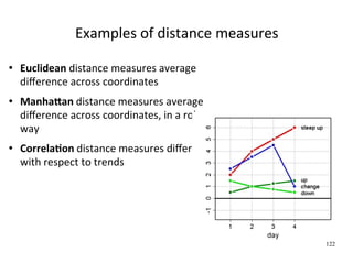
123. Comparison of the distances
All distances are normalized to the interval
[0,10] and then rounded
123

124. Clustering algorithms
 Popular algorithms for clustering
 hierarchical clustering
 K‐means
 SOMs (Self‐Organizing Maps)
 autoclass, mixture models...
 Hierarchical clustering allows the choice of the dissimilarity
matrix.
 k‐Means and SOMs take original data directly as input.
AXributes are assumed to live in Euclidean space.
124

125. Hierarchical clustering
AgglomeraWve clustering:
1. Each object is assigned to its own cluster
2. IteraWvely:
 the two most similar clusters are joined and replaced by
a new one
 the distance matrix is updated with this new cluster
replacing the two joined clusters
(divisive clustering would start from a big cluster)
125

126. Distance between two clusters
 Single linkage uses the smallest distance
 Complete linkage uses the largest distance
 Average linkage uses the average distance
126

127. Hierarchical clustering
(wikipedia)
127

128. Dendrogram
 Hierarchical clustering are visualized through dendrograms
 Clusters that are joined are combined by a line
 Height of line is distance between clusters
 Can be used to determine visually the number of clusters
128

129. IllustraWons (1)
 Breast cancer data (Langerød
et al., Breast cancer, 2007)
 80 tumor samples (wild‐
type,TP53 mutated), 80 genes
129

130. IllustraWons (2)
Assfalg et al., PNAS, Jan 2008
 Evidence of different metabolic phenotypes in humans
 Urine samples of 22 volunteers over 3 months, NMR
spectra analysed by HCA
130

131. Hierarchical clustering
 Strengths
 No need to assume any parWcular number of clusters
 Can use any distance matrix
 Find someWmes a meaningful taxonomy
 LimitaWons
 Find a taxonomy even if it does not exist
 Once a decision is made to combine two clusters it cannot be
undone
 Not well theoreWcally moWvated
131

132. k‐Means clustering
 ParWWoning algorithm with a prefixed number k of clusters
 Use Euclidean distance between objects
 Try to minimize the sum of intra‐cluster variances
k
∑ ∑ d 2  o,c j 
j= 1 o∈Cluster j
where cj is the center of cluster j and d2 is the Euclidean
distance
132

133. k‐Means clustering
133

134. k‐Means clustering
134

135. k‐Means clustering
135

136. k‐Means clustering
 Strengths
 Simple, understandable
 Can cluster any new point (unlike hierarchical clustering)
 Well moWvated theoreWcally
 LimitaWons
 Must fix the number of clusters beforehand
 SensiWve to the iniWal choice of cluster centers
 SensiWve to outliers
136

137. SubopWmal clustering
 You could obtain any of these from a random start of k‐
means
 SoluWon: restart the algorithm several Wmes
137

138. ApplicaWon: vector quanWzaWon
138

139. Principal Component Analysis
 An exploratory technique used to reduce the
dimensionality of the data set to a smaller space (2D, 3D)
A1 A2 A3 A4 A5 A6 A7 A8 A9 A10
PC1 PC2
0.25 0.93 0.04 -0.78 -0.5 3 0.57 0.19 0.29 0.37 -0.22 0 .3 6 0 .1
-2.3 -1.2 -4.5 -0.51 -0.7 6 0.07 0.81 0.95 0.99 0.26 -2 .3 -1 .2
-0.29 -1 0.73 -0.33 0 .52 0.13 0.13 0.53 -0.5 -0.48 0 .2 7 -0 .8 9
-0.16 -0.17 -0.26 0 .32 -0.0 8 -0 .38 -0 .48 0.99 -0.95 0.34 -0 .1 9 0 .7
0.07 -0.87 0.39 0.5 -0.6 3 -0 .53 0.79 0.88 0.74 -0.14 -0 .7 7 -0 .7
0.61 0.15 0.68 -0.94 0 .5 0.06 -0 .56 0.49 0 -0.77 -0 .6 5 -0 .9 9
 Transform some large number of variables into a smaller
number of uncorrelated variables called principal
components (PCs)
139

140. ObjecWves of PCA
 Reduce dimensionality (pre‐processing for other methods)
 Choose the most useful (informaWve) variables
 Compress the data
 Visualize mulWdimensional data
 to idenWfy groups of objects
 to idenWfy outliers
140

141. Basic idea
 Goal: map data points into a few dimensions while trying to
preserve the variance of the data as much as possible
First
component
Second
component
141

142. Each component is a linear combinaWon of the
original variables
A1 A2 A3 A4 A5 A6 A7 A8 A9 A10 PC1 PC2
-0.39 -0.38 0.29 0 .65 0 .15 0.73 -0 .57 0.91 -0.89 -0.17 0 .6 2 -0 .3 3
-2.3 -1.2 -4.5 -0.15 0 .86 -0 .85 0.43 -0.19 -0.83 -0.4 -2 .3 -1 .2
0 .9 0 .4 -0.11 0 .62 0 .94 0.97 0.1 -0.41 0.01 0.1 0 .8 8 0 .3 1
-0.82 -0.31 0.14 0 .22 -0.4 9 -0 .76 0.27 0 -0.43 -0.81 -0 .1 8 -0 .0 5
0.71 0.39 -0.09 0 .26 -0.4 6 -0 .05 0.46 0.39 -0.01 0.64 -0 .3 9 -0 .0 1
-0.25 0.27 -0.81 -0.42 0 .62 0.54 -0 .67 -0.15 -0.46 0.69 -0 .6 1 0 .5 3
Scores for each
sample and PC
PC1=0.2*A1+3.4*A2-4.5*A3 VAR(PC1)=4.5  45%
PC2=0.4*A4+5.6*A5+2.3*A7 VAR(PC2)=3.3  33%
... ...
Loading of a variable For each component, we
 Gives an idea of its importance in have a measure of the
the component percentage of the variance
 Can be use for feature selection of the initial data that it
contains
142

143. MathemaWcally (FYI)
 Given a data matrix X (nxd, n samples, d variables)
 Normalize X by substracWng mean from each data point
 Construct a covariance matrix C=XTX/n (dxd)
 Calculate the eigenvectors and eigenvalues of the C
 Sort eigenvectors by eigenvalues in decreasing order
 Map data point x to the direcWon v by compuWng the dot
product
143

144. IllustraWon (1/3)
Holmes et al., Nature, Vol. 453, No. 15, May 2008
 InvesWgaWon of metabolic phenotype variaWon across and
within four human populaWons (17 ciWes from 4 countries:
China, Japan, UK, USA)
1
 H NMR spectra of urine specimens from 4630 parWcipants
 PCA plots of median spectra per populaWon (city) and
gender
144

145. Holmes et al., Nature, Vol. 453, No. 15, May 2008
145

146. IllustraWon (2/3)
Neuroimaging
L voxels (brain regions)
A1 A2 A3 A4 A5 ... A7 A8
-0 . 9 1 0 .7 4 0 .7 4 0 .9 7 -0 .0 6 ... -0 .0 4 -0 . 7 3
-2 .3 -1 .2 -4 . 5 0 .4 7 0 .1 3 ... 0 .1 6 0 .2 6
-0 . 9 8 -0 . 4 6 0 .9 8 0 .7 7 -0 .1 4 ... 0 .4 4 -0 . 1 2
0 .9 7 -0 . 6 4 -0 . 3 -0 .1 4 -0 .2 9 ... -0 .4 3 0 .2 7
-0 . 6 4 -0 . 3 4 0 .2 1 -0 .5 7 -0 .3 9 ... 0 .0 2 -0 . 6 1
0 .4 1 -0 . 9 5 0 .2 1 -0 .1 7 -0 .6 8 ... 0 .1 1 0 .4 9
N patients/brain maps
146

147. Books
 Reference book:
 The elements of staEsEcal learning: data mining, inference, and predicEon. T.
HasWe et al, Springer, 2001 (second ediWon in 2008)
 Downloadable (with a Ulg connecWon) from
 hXp://www.springerlink.com/content/978‐0‐387‐84857‐0
 Other textbooks
 PaFern RecogniEon and Machine Learning (InformaEon Science and StaEsEcs).
C.M.Bishop, Springer, 2004
 PaFern classificaEon (2nd ediWon). R.Duda, P.Hart, D.Stork, Wiley Interscience,
2000
 IntroducEon to Machine Learning. Ethan Alpaydin, MIT Press, 2004.
 Machine Learning. Tom Mitchell, McGraw Hill, 1997.
147

148. Books
 More advanced topics
 kernel methods for paFern analysis. J. Shawe‐Taylor and N. CrisWanini.
Cambridge University Press, 2004
 Reinforcement Learning: An IntroducEon. R.S. SuXon and A.G. Barto. MIT Press,
1998
 Neuro‐Dynamic Programming. D.P Bertsekas and J.N. Tsitsiklis. Athena
ScienWfic, 1996
 Semi‐supervised learning. Chapelle et al., MIT Press, 2006
 PredicEng structured data. G. Bakir et al., MIT Press, 2007
148

149. SoFwares
 Pepito
 www.pepite.be
 Free for academic research and educaWon
 WEKA
 hXp://www.cs.waikato.ac.nz/ml/weka/
 Many R and Matlab packages
 hXp://www.kyb.mpg.de/bs/people/spider/
 hXp://www.cs.ubc.ca/~murphyk/SoFware/BNT/bnt.html
149

150. Journals
 Journal of Machine Learning Research
 Machine Learning
 IEEE TransacWons on PaXern Analysis and Machine Intelligence
 Journal of ArWficial Intelligence Research
 Neural computaWon
 Annals of StaWsWcs
 IEEE TransacWons on Neural Networks
 Data Mining and Knowledge Discovery
 ...
150

151. Conferences
 InternaWonal Conference on Machine Learning (ICML)
 European Conference on Machine Learning (ECML)
 Neural InformaWon Processing Systems (NIPS)
 Uncertainty in ArWficial Intelligence (UAI)
 InternaWonal Joint Conference on ArWficial Intelligence (IJCAI)
 InternaWonal Conference on ArWficial Neural Networks (ICANN)
 ComputaWonal Learning Theory (COLT)
 Knowledge Discovery and Data mining (KDD)
 ...
151