The document is a practical report on designing various finite impulse response (FIR) filters using LabVIEW, covering low pass and band pass filters with specific parameters. It includes detailed steps for calculating filter coefficients, applying window functions, and provides a list of available filter icons in LabVIEW for digital signal processing. Additionally, it discusses different types of filters and commonly used window functions in filter design.

1. 1 | P a g e
A
Practical Report
on
INTRODUCTION TO FILTERS
Under LabVIEW Environment
Submitted To: Submitted By:
Mr. Raj Kumar Garg Paramjeet Singh Jamwal
Assistant Professor PG/ICE/136321
LabVIEW
M.Tech (ICE)
Third Semester
Department of Electrical and Instrumentation Engineering
Sant Longowal Institute of Engineering and Technology
Longowal – 148106 (INDIA)
Nov 2014

2. 2 | P a g e
CONTENT
S. No. Example Page No.
1. Design a Finite Impulse Response Low Pass Filter using rectangular
window with a cut off frequency of 1 KHz and sampling rate of 4
KHz with 11 samples.
LabVIEW
3.
2. Design a Finite Impulse Response Band Pass Filter using Triangular
(Bartlett) window with a lower cut off frequency of 3 KHz, higher
cut off frequency of 5.5 KHz and sampling rate of 20 KHz with 15
samples (Order-14).
5.
3. Type of filter and commonly used Windows. 7.
4. List of filter icon available in the LabVIEW. 8.

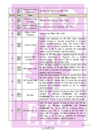
3. 1. Design a Finite Impulse Response Low Pass Filter using rectangular window with a cut off
3 | P a g e
frequency of 1 KHz and sampling rate of 4 KHz with 11 samples.
1 −휔푐 ≤ 휔 ≤ 휔푐
0 −
휔푐
LabVIEW
Given:
Fs : 4 KHz
fc : 1 KHz
N : 11
Step: 1 - Finding Hd(ωt):
퐻푑 (휔푇) =
[
휔푠
2
≤ 휔 ≤ −휔푐
0 휔푐 ≤ 휔 ≤
휔푠
2 ]
휔푠 = 2휋푓푠 = 25132.74 푟푎푑/푠푒푐
푇 =
1
푓푠
= 0.25 ∗ 10−3푠푒푐
Step: 2 – Finding hd(n):
ℎ푑 (푛) =
1
휔푠
∫ 푒푗휔푛푇 . 푑휔
−휔푐
ℎ푑 (푛) =
2
휔푠 푛푇
∗ 푆푖푛(휔푐 푛푇)
ℎ푑 (푛) =
푆푖푛(휔푐 푛푇)
휋푛
; 푤ℎ푒푛 푛 ≠ 0
ℎ푑 (푛) =
2휔푐
휔푠
; 푤ℎ푒푛 푛 = 0
Step: 3 – Window Function:
휔푟 (푛) = [
1 푓표푟 푛 = 0 푡표 푀 − 1
0 표푡ℎ푒푟푤푖푠푒
]
Step: 4 – Coefficients:
hd(n) 0.5 0.3183 0 -0.1061 0 0.0637 -0.0455 0 0.0354 0
ωr(n) 1 1 1 1 1 1 1 1 1 1
h(n) 0.5 0.3183 0 -0.1061 0 0.0637 -0.0455 0 0.0354 0

4. 4 | P a g e
LabVIEW
Step: 5.1 – Block Diagram:
Step: 5.2 – Front Panel:
Reference: Salivahnan S., Ghananpriya C., “Digital Signal Processing”, 2nd Edition, pp-439-440,
Example-7.4.

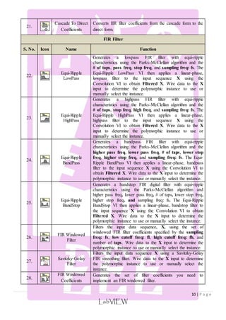
5. 2. Design a Finite Impulse Response Band Pass Filter using Triangular (Bartlett) window with a
lower cut off frequency of 3 KHz, higher cut off frequency of 5.5 KHz and sampling rate of 20
KHz with 15 samples (Order-14).
5 | P a g e
푆푖푛(휔푐1(푛 − 푀))
LabVIEW
Given:
Fs : 20 KHz
fcl : 3 KHz
fch : 5.5 KHz
N : 15
Step: 1 – Finding hd(n):
ℎ푑 (푛) = [
휋 (푛 − 푀)
−
푆푖푛(휔푐2(푛 − 푀))
휋(푛 − 푀)
푛 ≠ 푀
1 −
휔푐2−휔푐1
휋
푛 = 푀
]
Where: M index of middle coefficient.
휔푐1 =
2휋푓푐1
푓푠
= 0.3휋
휔푐2 =
2휋푓푐2
푓푠
= 0.55휋
Step: 2 – Window Function:
휔[푛] = [
2푛
푁 − 1
; 푓표푟 0 ≤ 푛 ≤ 푡표
푁 − 1
2
2 −
2푛
푁 − 1
;
푁 + 1
2
≤ 푛 ≤ 푁 − 1
]
Step: 3 – Coefficients:
Coefficient 0 1 2 3 4 5 6 7
hd(n) 0.034696 0.011737 -0.10868 -0.09355 0.127326 0.200547 -0.05687 0.75
ωr(n) 0 0.142857 0.285714 0.428571 0.571429 0.714286 0.857143 1
h(n) 0 0.001677 -0.03105 -0.04009 0.072758 0.143248 -0.048747 0.75
Coefficient 8 9 10 11 12 13 14
hd(n) 0.056872 -0.20055 -0.12733 0.093549 0.108678 -0.01174 -0.034696
ωr(n) 0.857143 0.714286 0.571429 0.428571 0.285714 0.142857 0
h(n) -0.048747 0.143248 0.072758 -0.040092 -0.031051 0.001667 0

6. 6 | P a g e
LabVIEW
Step: 4.1 – Block Diagram:
Step: 4.2 – Front Panel:
Reference: “Mikro Elektronika”, http://www.mikroe.com/chapters/view/72/chapter-2-fir-filters/.

7. 7 | P a g e
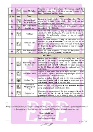
3. Type of filter and commonly used Windows.
S.No. Type of Filter Frequency Response hd[n]
푆푖푛(휔푐 (푛 − 푀))
1. Low Pass Filter ℎ푑 (푛) = [
0.54 + 0.46 ∗ 퐶표푠
LabVIEW
휋(푛 − 푀)
푛 ≠ 푀
휔푐
휋
푛 = 푀
]
2. High Pass Filter ℎ푑 (푛) = [
1 −
휔푐
휋
푛 ≠ 푀
−
푆푖푛(휔푐 (푛 − 푀))
휋(푛 − 푀)
푛 = 푀
]
3. Band Pass Filter ℎ푑 (푛) = [
푆푖푛(휔푐2(푛 − 푀))
휋(푛 − 푀)
−
푆푖푛(휔푐1(푛 − 푀))
휋(푛 − 푀)
푛 ≠ 푀
휔푐2− 휔푐1
휋
푛 = 푀
]
4. Band Stop Filter ℎ푑 (푛) = [
푆푖푛(휔푐1(푛 − 푀))
휋(푛 − 푀)
−
푆푖푛(휔푐2(푛 − 푀))
휋(푛 − 푀)
푛 ≠ 푀
1 −
휔푐2− 휔푐1
휋
푛 = 푀
]
S. No. Window Function
1. Triangular (Bartlett) 푊푇 [푛] =
2|푛|
푀 − 1
; 푓표푟 |푛| ≤ 푀 − 1
2. Hanning 푊ℎ푛 =
1
2
[1 −
퐶표푠2휋푛
푀 − 1
] ;
3. Hamming 푊퐻푚 = [
2휋푛
푀 − 1
; |푛| ≤ 푄
0; 푒푙푒푠푤ℎ푒푟푒
]
4. Blackman 푊퐵 [푛] = 0.42 + 0.5 ∗ 퐶표푠
2휋푛
푀 − 1
+ 0.08 ∗ 퐶표푠
4휋푛
푀 − 1
5. Kaiser 푊푘 [푛] = [
퐼표(훽)
퐼표(훼)
|푛| ≤ 푄
0; 푒푙푒푠푤ℎ푒푟푒
]

8. 8 | P a g e
4. List of filter icon available in the LabVIEW.
Filter icon is available at Functions/Signal Processing/Filters.
IIR Filter
S. No. Icon Name Function
LabVIEW
01.
Butterworth Filter
Generates a digital Butterworth filter by calling the
Butterworth Coefficients VI. Wire data to the X input to
determine the polymorphic instance to use or manually
select the instance.
02.
Chebyshev Filter
Generates a digital Chebyshev filter by calling the
Chebyshev Coefficients VI. Wire data to the X input to
determine the polymorphic instance to use or manually
select the instance.
03.
Inverse Chebyshev
Filter
Generates a digital Chebyshev II filter by calling the Inv
Chebyshev Coefficients VI. Wire data to the X input to
determine the polymorphic instance to use or manually
select the instance.
04.
Elliptic Filter
Generates a digital elliptic filter by calling the Elliptic
Coefficients VI. Wire data to the X input to determine the
polymorphic instance to use or manually select the instance.
05.
Bessel Filter
Generates a digital Bessel filter by calling the Bessel
Coefficients VI. Wire data to the X input to determine the
polymorphic instance to use or manually select the instance.
06.
Butterworth
Coefficients
Generates the set of filter coefficients to implement an IIR
filter as specified by the Butterworth filter model. You can
pass these filter coefficients, IIR Filter Cluster, to the IIR
Cascade Filter VI to filter a sequence of data.
07.
Chebyshev
Coefficients
Generates the set of filter coefficients to implement an IIR
filter as specified by the Chebyshev filter model. You can
pass these coefficients to the IIR Cascade Filter VI to filter
a sequence of data.
08.
Inv Chebyshev
Coefficients
Generates the set of filter coefficients to implement an IIR
filter as specified by the Chebyshev II Filter model. You
can pass these coefficients to the IIR Cascade Filter VI to
filter a sequence of data.
09.
Elliptic
Coefficients
Generates the set of filter coefficients to implement a digital
elliptic IIR filter. You can pass these coefficients to the IIR
Cascade Filter VI.
10.
Bessel
Coefficients
Generates the set of filter coefficients to implement an IIR
filter as specified by the Bessel filter model. You then can
pass these coefficients to the IIR Cascade Filter VI.

9. 9 | P a g e
LabVIEW
11.
Butterworth Order
Estimation
Estimates the Butterworth filter order.
S. No. Icon Name Function
12.
Chebyshev Order
Estimation
Estimates the Chebyshev I filter order.
13.
Inverse Chebyshev
Order Estimation
Estimates the Inverse Chebyshev filter order.
14.
Elliptic Order
Estimation
Estimates the Elliptic filter order.
15.
Inverse f Filter
Designs and implements an IIR filter whose magnitude-squared
response is inversely proportional to frequency
over a specified frequency range. This inverse-f filter is
typically used to colorize spectrally flat, or white, noise.
Wire data to the X input to determine the polymorphic
instance to use or manually select the instance.
16.
Inverse f Filter
Coefficients
Designs an IIR filter whose magnitude-squared response is
inversely proportional to frequency over a specified
frequency range. This inverse-f filter is typically used to
colorize spectrally flat, or white, noise.
17.
IIR Cascade Filter
Filters the input sequence X using the cascade form of the
IIR filter specified by the IIR Filter Cluster. Wire data to
the X input to determine the polymorphic instance to use or
manually select the instance.
18.
IIR Cascade Filter
with I.C.
Filters the input sequence X using the cascade form of the
IIR filter specified by the IIR Filter Cluster. This VI is
similar to the IIR Cascade Filter VI except that you specify
the initial conditions for this VI. Wire data to the X input to
determine the polymorphic instance to use or manually
select the instance.
19.
IIR Filter
Filters the input sequence X using the direct form IIR filter
specified by Reverse Coefficients and Forward
Coefficients. Wire data to the X input to determine the
polymorphic instance to use or manually select the instance.
20.
IIR Filter with I.C.
Filters the input sequence X using the direct form IIR filter
specified by Reverse Coefficients and Forward
Coefficients. You can use this VI to process blocks of
continuous data. This VI is similar to the IIR Filter VI
except that you specify the initial conditions for this VI.
Wire data to the X input to determine the polymorphic
instance to use or manually select the instance.

10. 10 | P a g e
LabVIEW
21.
Cascade To Direct
Coefficients
Converts IIR filter coefficients from the cascade form to the
direct form.
FIR Filter
S. No. Icon Name Function
22.
Equi-Ripple
LowPass
Generates a lowpass FIR filter with equi-ripple
characteristics using the Parks-McClellan algorithm and the
# of taps, pass freq, stop freq, and sampling freq: fs. The
Equi-Ripple LowPass VI then applies a linear-phase,
lowpass filter to the input sequence X using the
Convolution VI to obtain Filtered X. Wire data to the X
input to determine the polymorphic instance to use or
manually select the instance.
23.
Equi-Ripple
HighPass
Generates a highpass FIR filter with equi-ripple
characteristics using the Parks-McClellan algorithm and the
# of taps, stop freq, high freq, and sampling freq: fs. The
Equi-Ripple HighPass VI then applies a linear-phase,
highpass filter to the input sequence X using the
Convolution VI to obtain Filtered X. Wire data to the X
input to determine the polymorphic instance to use or
manually select the instance.
24.
Equi-Ripple
BandPass
Generates a bandpass FIR filter with equi-ripple
characteristics using the Parks-McClellan algorithm and the
higher pass freq, lower pass freq, # of taps, lower stop
freq, higher stop freq, and sampling freq: fs. The Equi-
Ripple BandPass VI then applies a linear-phase, bandpass
filter to the input sequence X using the Convolution VI to
obtain Filtered X. Wire data to the X input to determine the
polymorphic instance to use or manually select the instance.
25.
Equi-Ripple
BandStop
Generates a bandstop FIR digital filter with equi-ripple
characteristics using the Parks-McClellan algorithm and
higher pass freq, lower pass freq, # of taps, lower stop freq,
higher stop freq, and sampling freq: fs. The Equi-Ripple
BandStop VI then applies a linear-phase, bandstop filter to
the input sequence X using the Convolution VI to obtain
Filtered X. Wire data to the X input to determine the
polymorphic instance to use or manually select the instance.
26.
FIR Windowed
Filter
Filters the input data sequence, X, using the set of
windowed FIR filter coefficients specified by the sampling
freq: fs, low cutoff freq: fl, high cutoff freq: fh, and
number of taps. Wire data to the X input to determine the
polymorphic instance to use or manually select the instance.
27.
Savitzky-Golay
Filter
Filters the input data sequence X using a Savitzky-Golay
FIR smoothing filter. Wire data to the X input to determine
the polymorphic instance to use or manually select the
instance.
28.
FIR Windowed
Coefficients
Generates the set of filter coefficients you need to
implement an FIR windowed filter.

11. 11 | P a g e
LabVIEW
29.
Parks-McClellan
Generates a set of linear-phase FIR multiband digital filter
coefficients using the # of taps, sampling frequency: fs,
Band Parameters, and filter type.
S. No. Icon Name Function
30.
Savitzky-Golay
Filter Coefficients
Designs a Savitzky-Golay FIR smoothing filter. This VI
returns the designed Savitzky-Golay filter coefficients and
the differentiation filter coefficients.
31.
FIR Narrowband
Coefficients
Generates a set of filter coefficients to implement a digital
interpolated FIR (IFIR) filter.
32.
FIR Filter
Filters the input sequence X using the direct-form FIR filter
specified by FIR Coefficients. Wire data to the X input to
determine the polymorphic instance to use or manually
select the instance.
33.
FIR Filter with
I.C.
Filters the input sequence X using the direct-form FIR filter
specified by FIR Coefficients. You can use this VI to
process blocks of continuous data. Wire data to the X input
to determine the polymorphic instance to use or manually
select the instance.
34.
FIR Narrowband
Filter
Filters the input sequence X using the interpolated FIR
(IFIR) filter specified by IFIR Coefficients.
Other Filter
35.
Smoothing Filter
Coefficients
Designs filter coefficients for a smoothing filter. You can
use this VI to design a moving-average FIR filter or an
exponentially-averaging IIR filter. The VI returns reverse
coefficients and forward coefficients for direct connection
to the IIR Filter VI, which is used to implement both FIR
and IIR filters.
36.
Zero Phase Filter
Applies a zero phase filter to an input sequence X. Wire
data to the X input to determine the polymorphic instance to
use or manually select the instance.
37.
Median Filter
Applies a median filter of rank to the input sequence X,
where rank is right rank if right rank is greater than zero,
or left rank if right rank is less than zero.
38.
Mathematical
Morphological
Filter
Filters the input data sequence X with Structure Element
using a mathematical morphological filter.
39.
Convolution
Computes the convolution of the input sequences X and Y.
Wire data to the X and Y inputs to determine the
polymorphic instance to use or manually select the instance.
---
An info4eee presentation, which provides Information for Electrical and Electronics Engineering students. It
is the initiative to share the material among the EEE students in a well mannered way.
Now available on:
info4eee.wordpress.com
facebook.com/info4eee