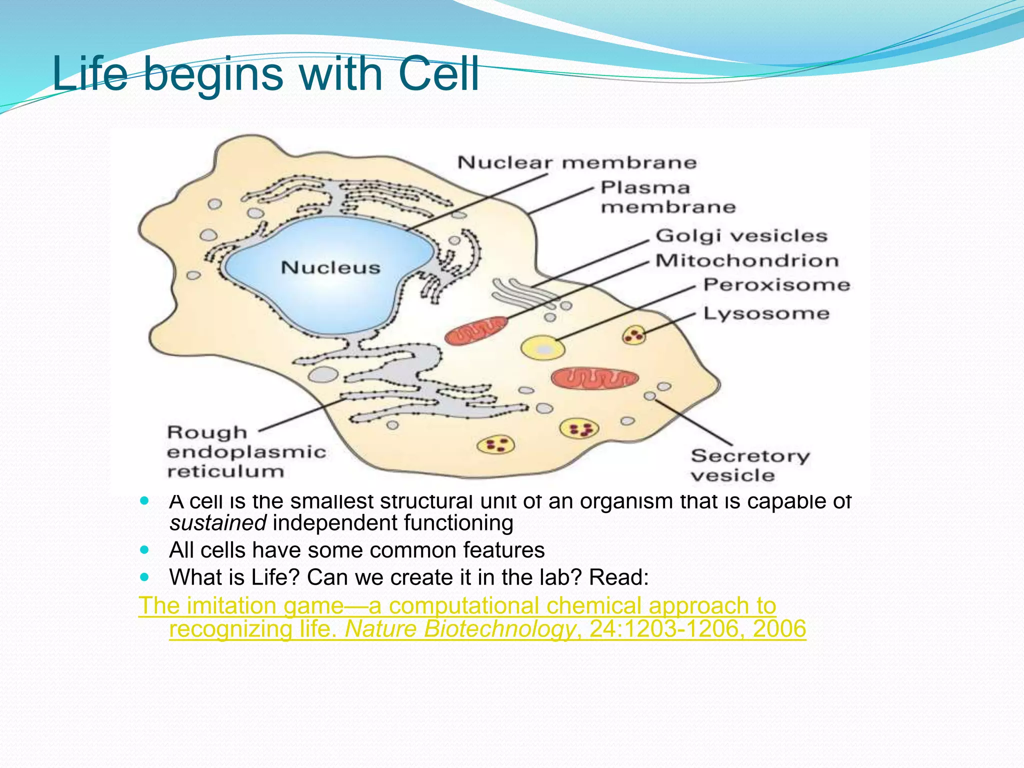
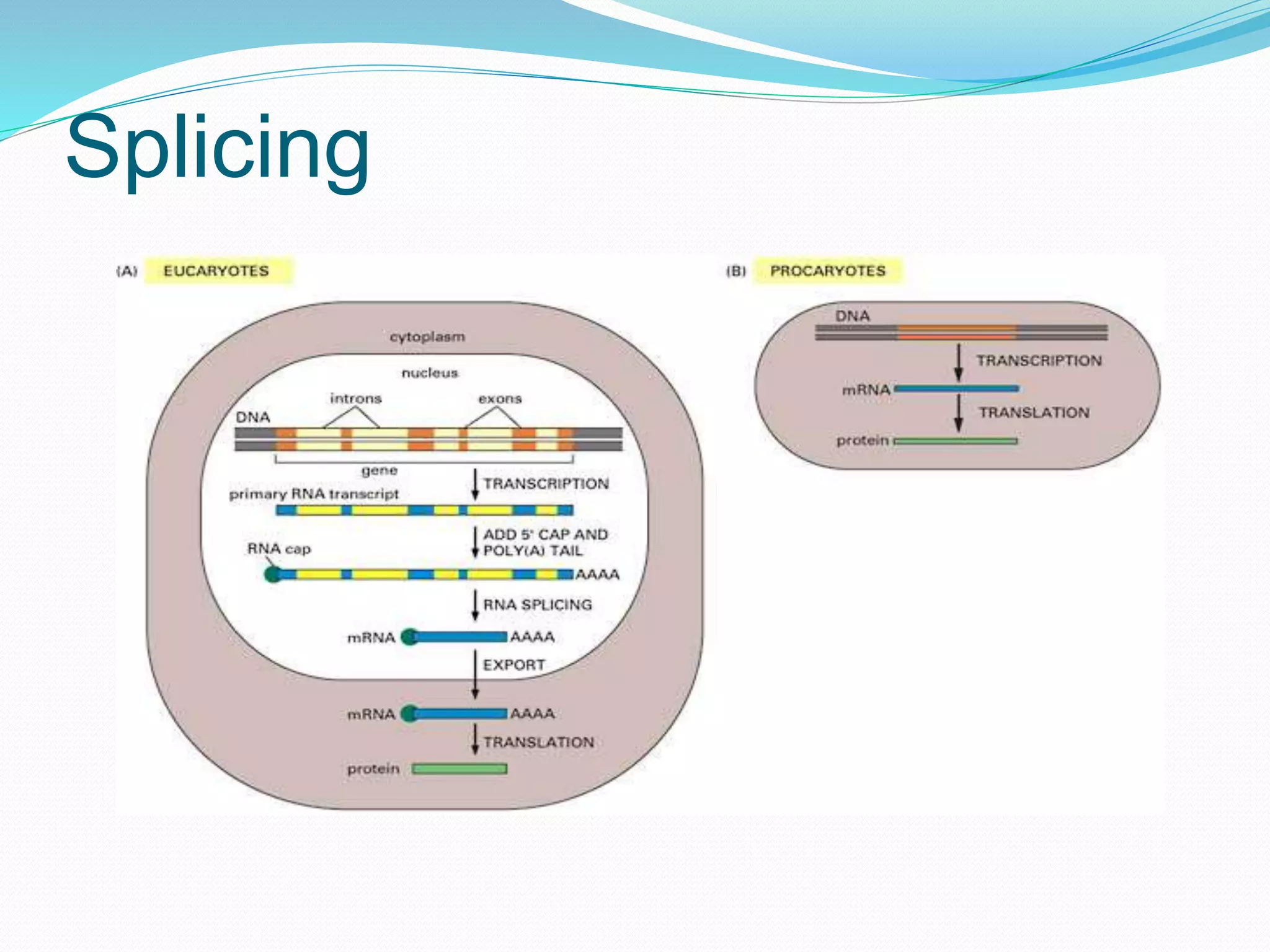
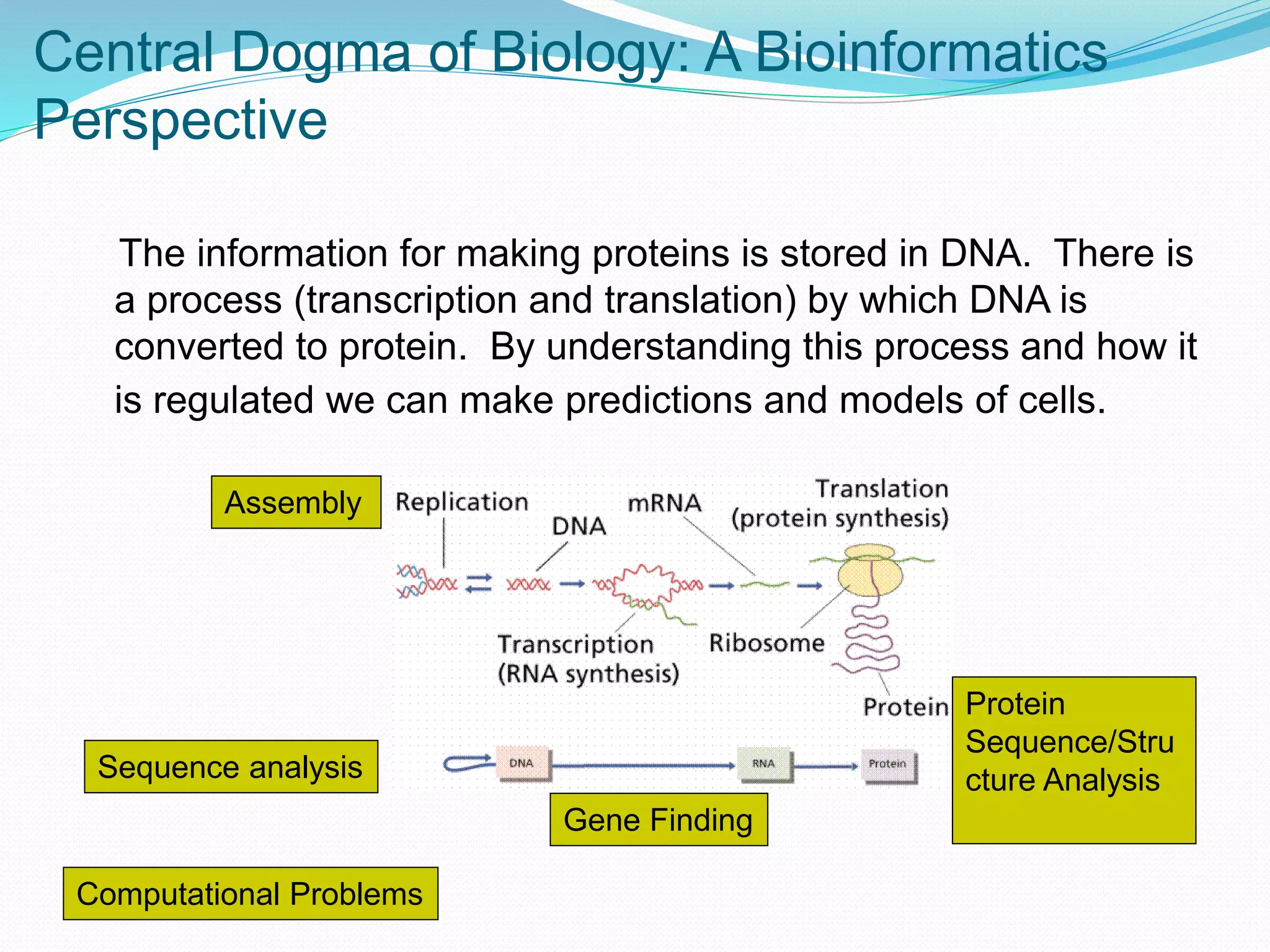
This document provides an overview of bioinformatics and related topics. It begins by defining bioinformatics as the use of computational techniques to understand biology. It then discusses the central dogma of biology, describing how DNA is transcribed into RNA and translated into protein. The document outlines common bioinformatics tasks like sequence analysis, databases, and modeling biological systems. It provides background on key biomolecules like DNA, RNA, and proteins and the information flow within biological systems.


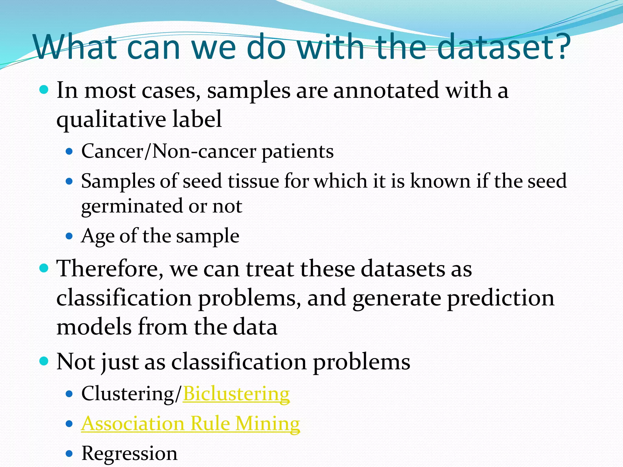
![Three case studies
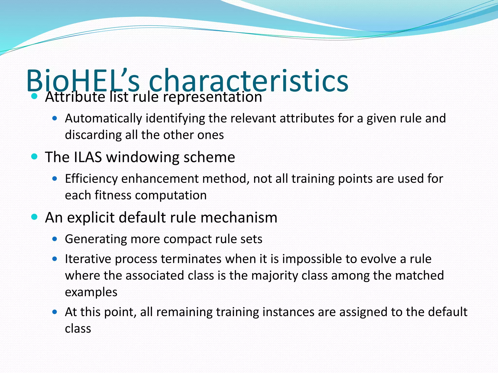
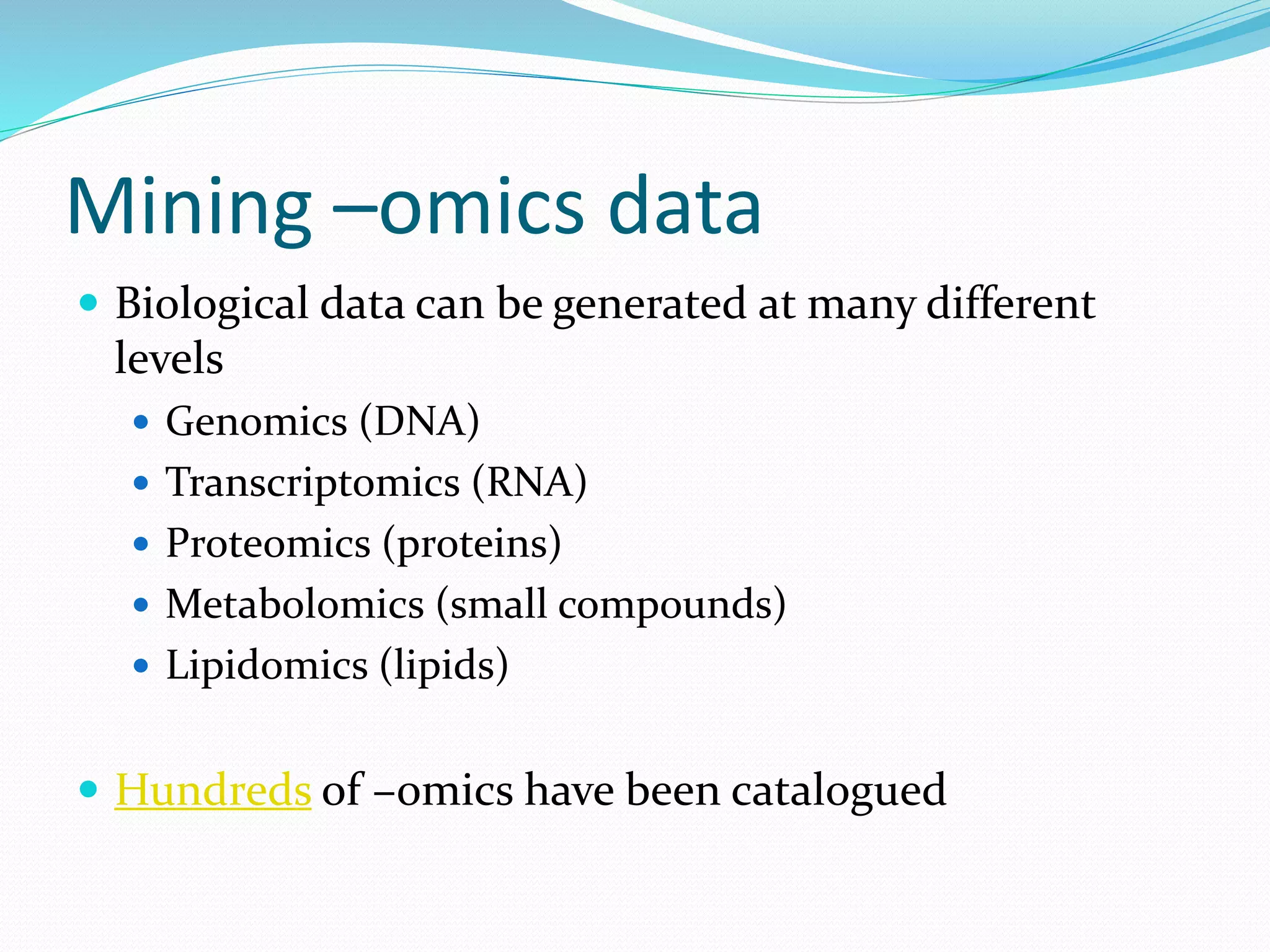
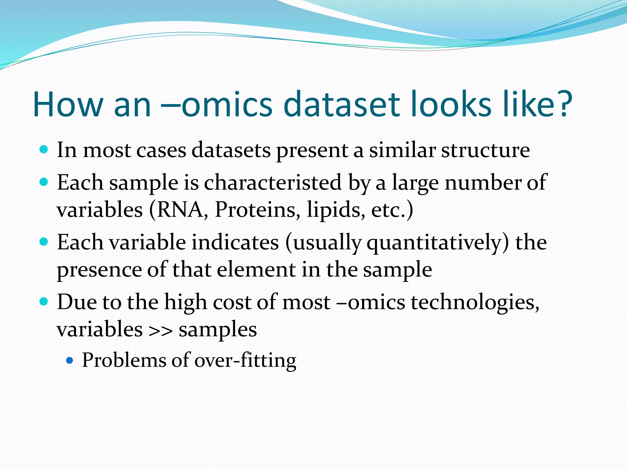
Mining –omics data
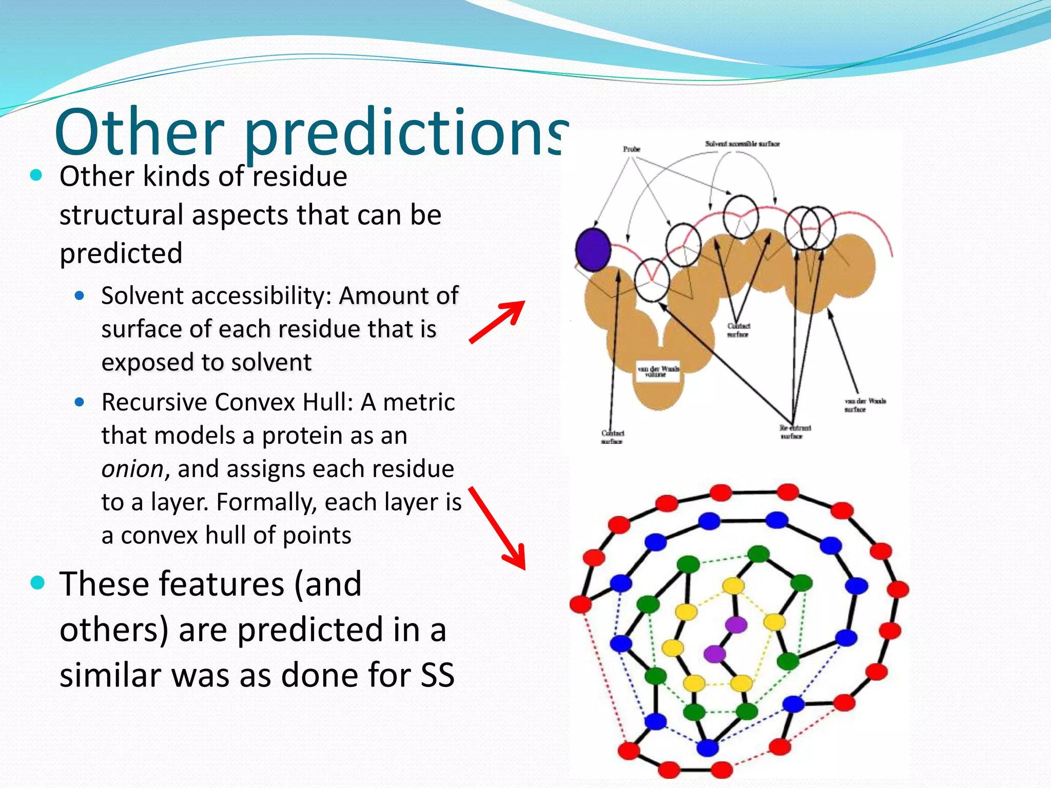
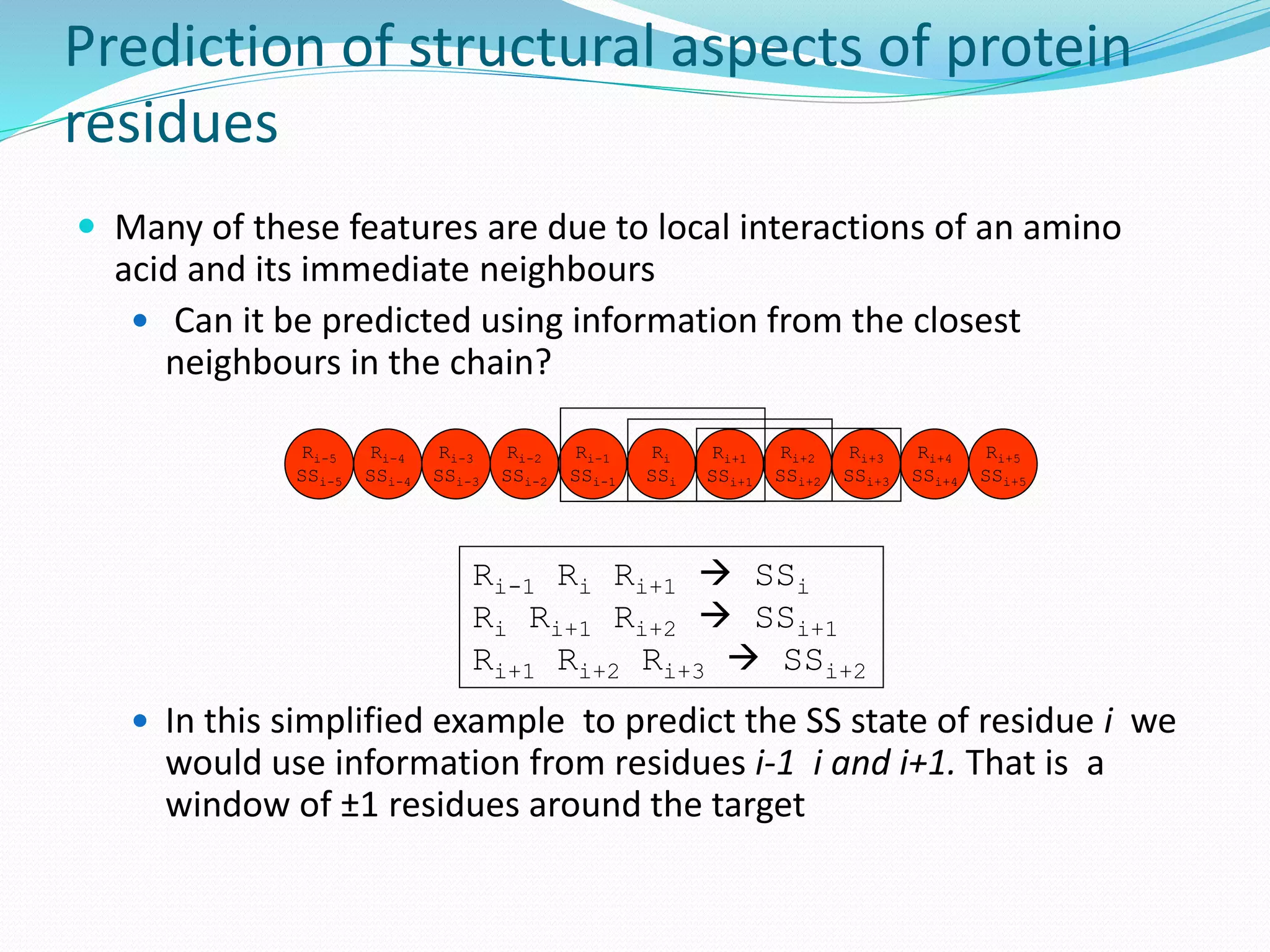
Predicting structural aspects of protein residues
Automated alphabet reduction for protein datasets
In all these three case studies we use the same
evolutionary learning system: BioHEL [Bacardit et al.,
09]](https://image.slidesharecdn.com/introduction-170331154845/75/Introduction-85-2048.jpg)
![BioHEL BioHEL [Bacardit et al., 09] is an evolutionary
learning system that applies the Iterative Rule
Learning (IRL) approach
Designed explicitly to deal with noisy large-scale
datasets
IRL was first used in EC by the SIA system
[Venturini, 93]](https://image.slidesharecdn.com/introduction-170331154845/75/Introduction-86-2048.jpg)


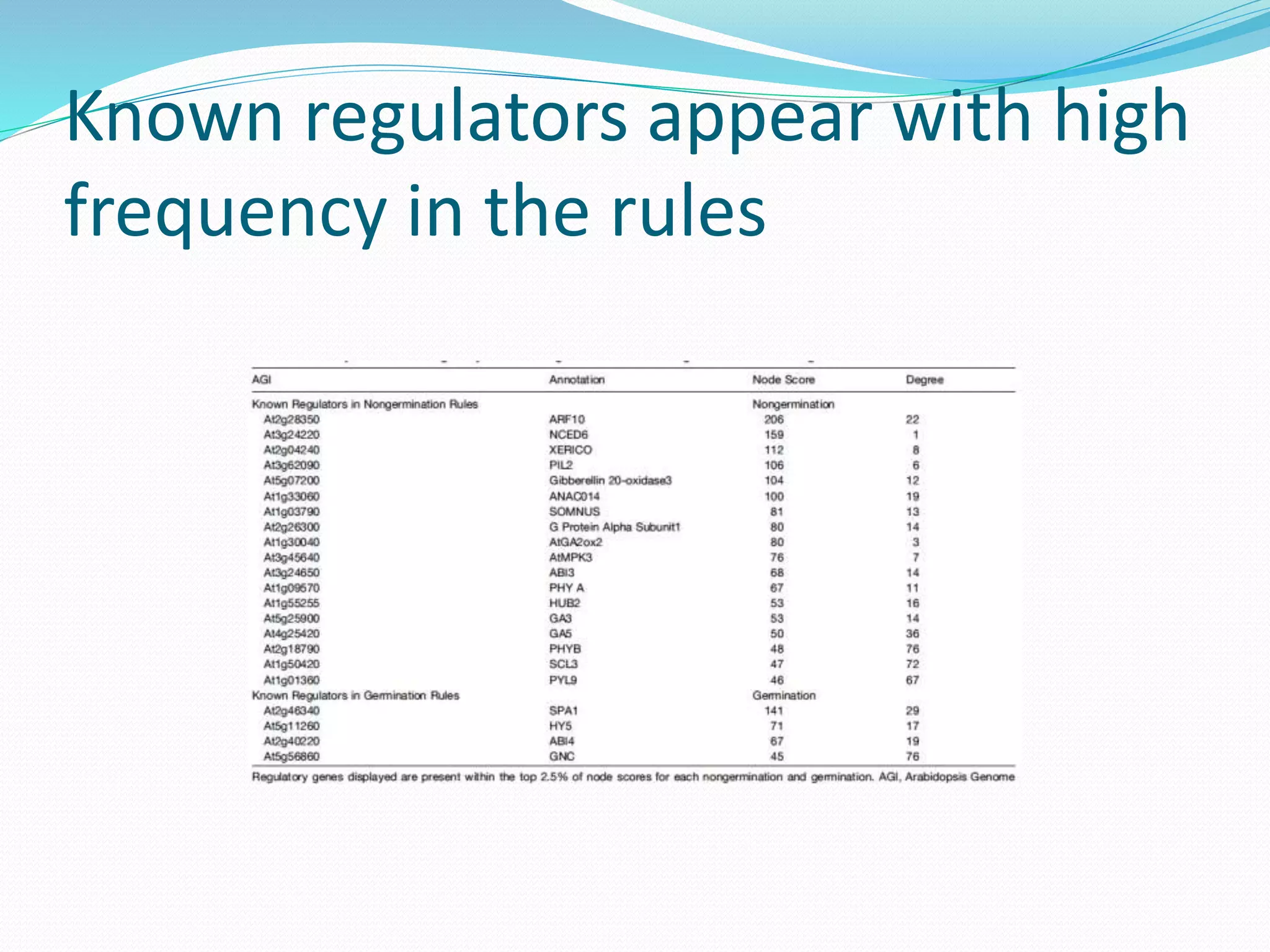
![Functional Network Reconstruction
for seed germination Microarray data obtained from seed tissue of Arabidopsis
Thaliana
122 samples represented by the expression level of
almost 14000 genes
It had been experimentally determined whether each of
the seeds had germinated or not
Can we learn to predict germination/dormancy from the
microarray data?
[Bassel et al., 2011]](https://image.slidesharecdn.com/introduction-170331154845/75/Introduction-97-2048.jpg)
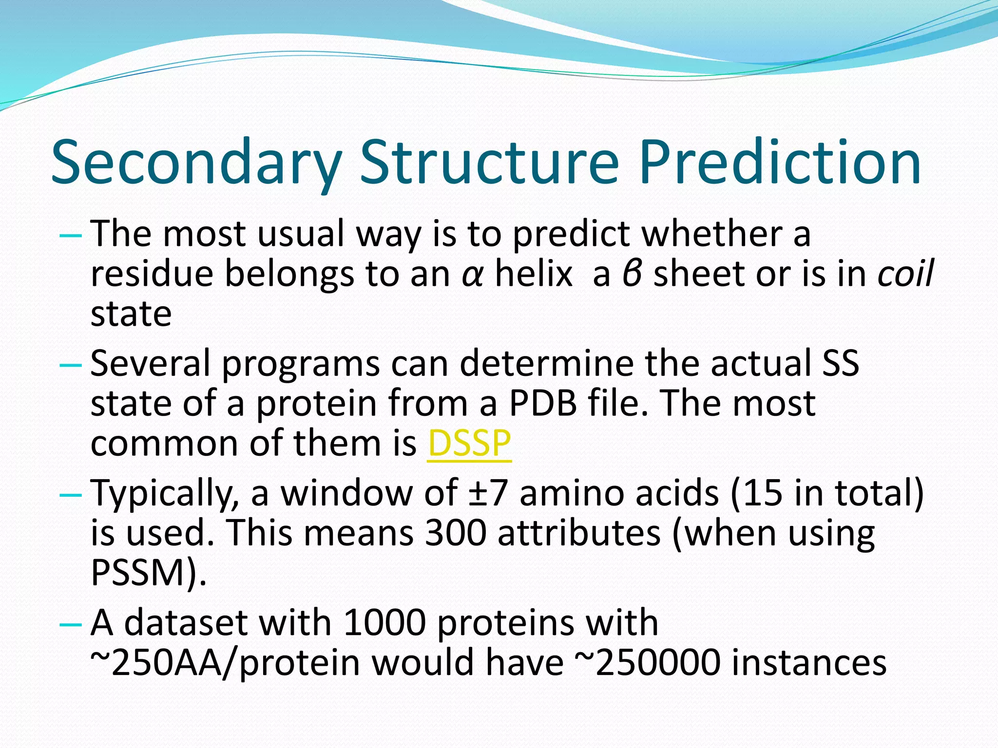
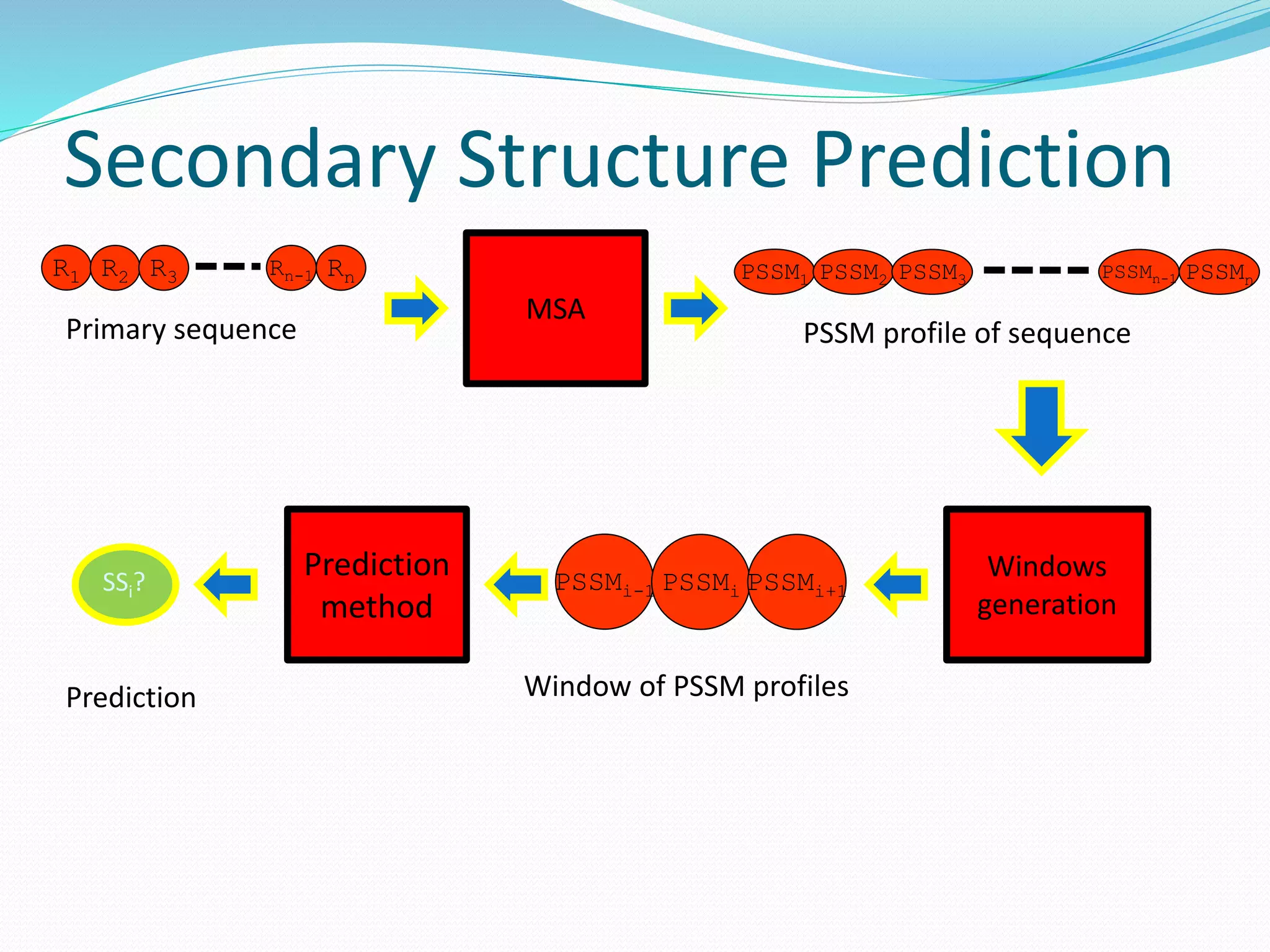
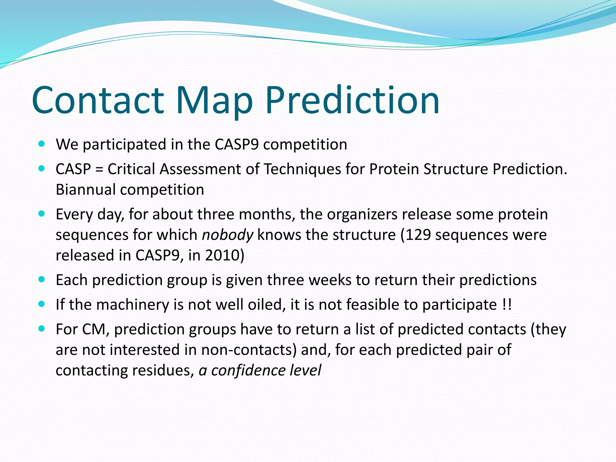

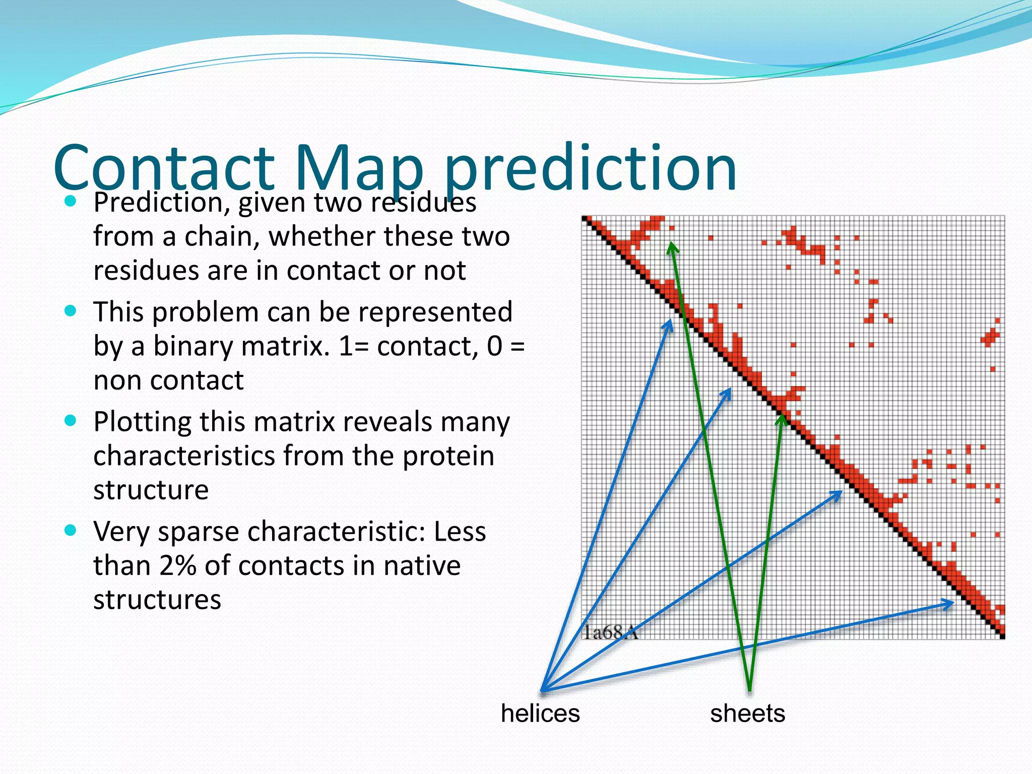
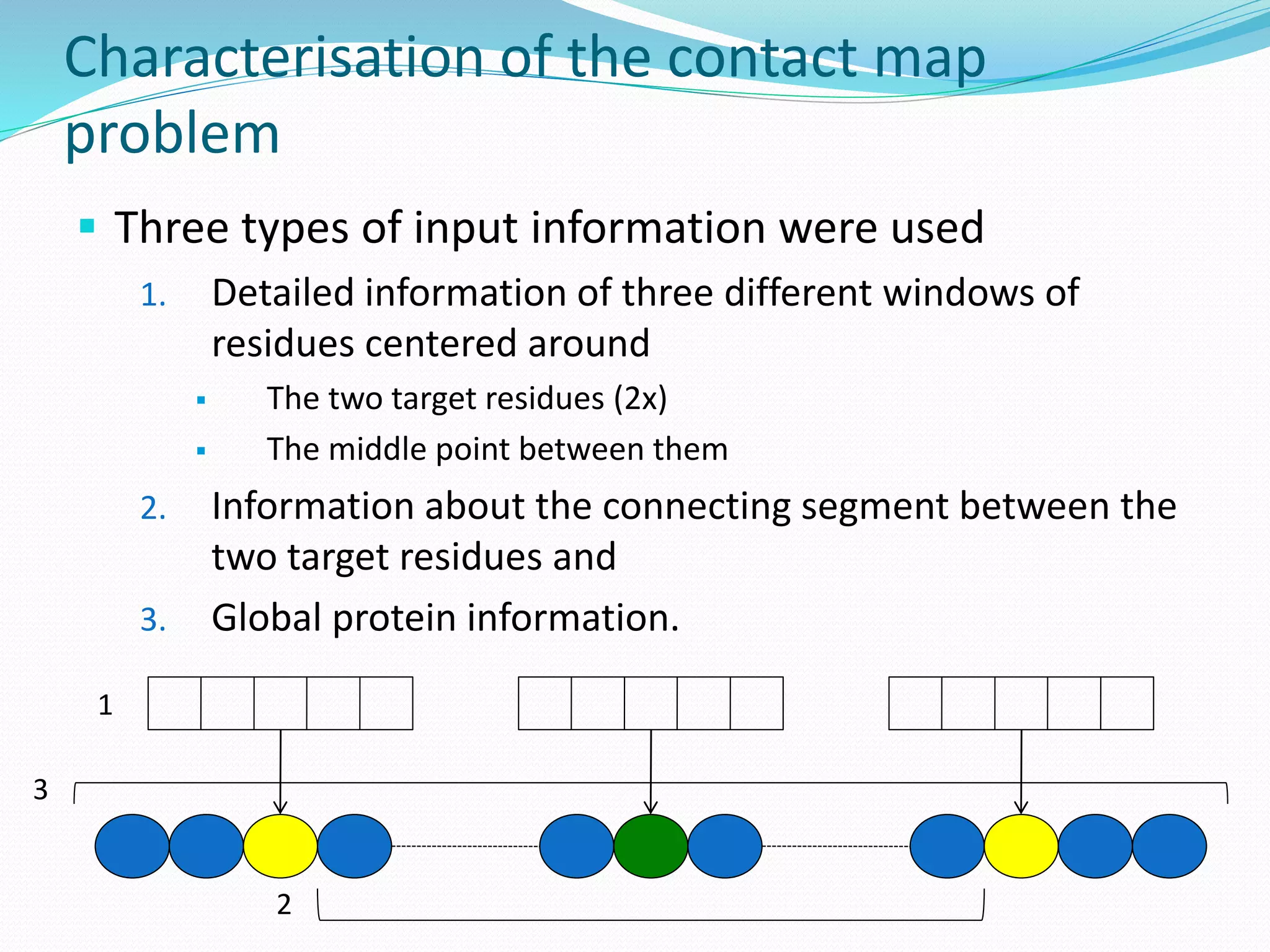
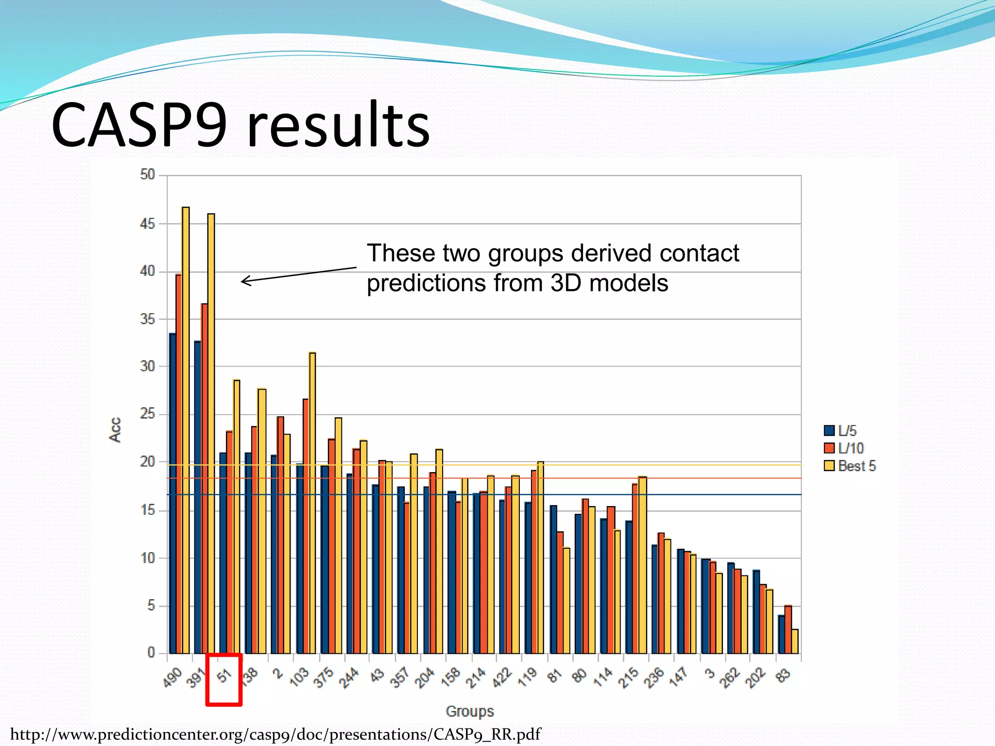
![Steps for CM prediction (Nottingham
method)
1. Prediction of
Secondary structure (using PSIPRED)
Solvent Accessibility
Recursive Convex Hull
Coordination Number
2. Integration of all these predictions plus other sources of
information
3. Final CM prediction (using BioHEL)
Using BioHEL [Bacardit et al., 09]](https://image.slidesharecdn.com/introduction-170331154845/75/Introduction-115-2048.jpg)

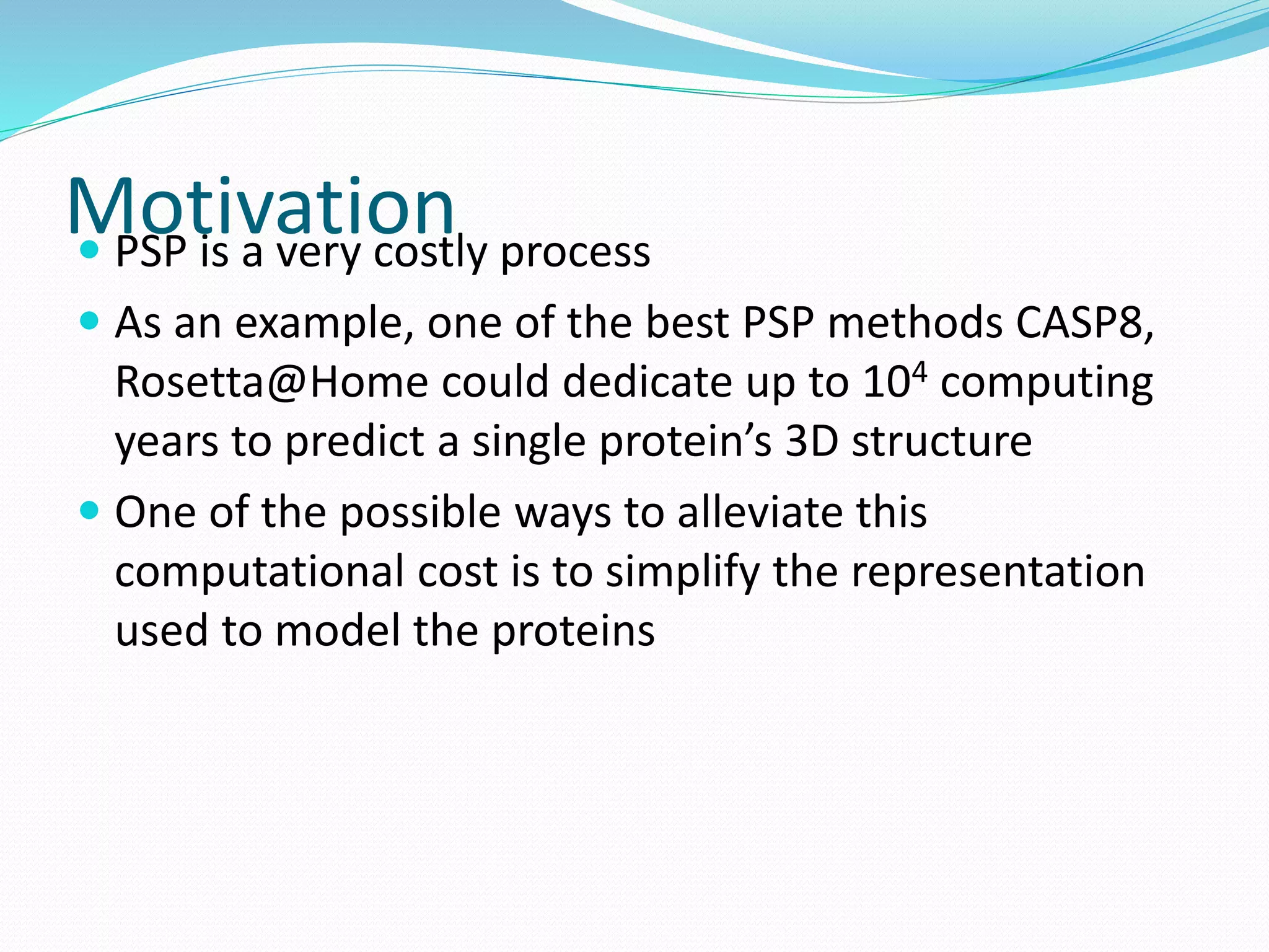
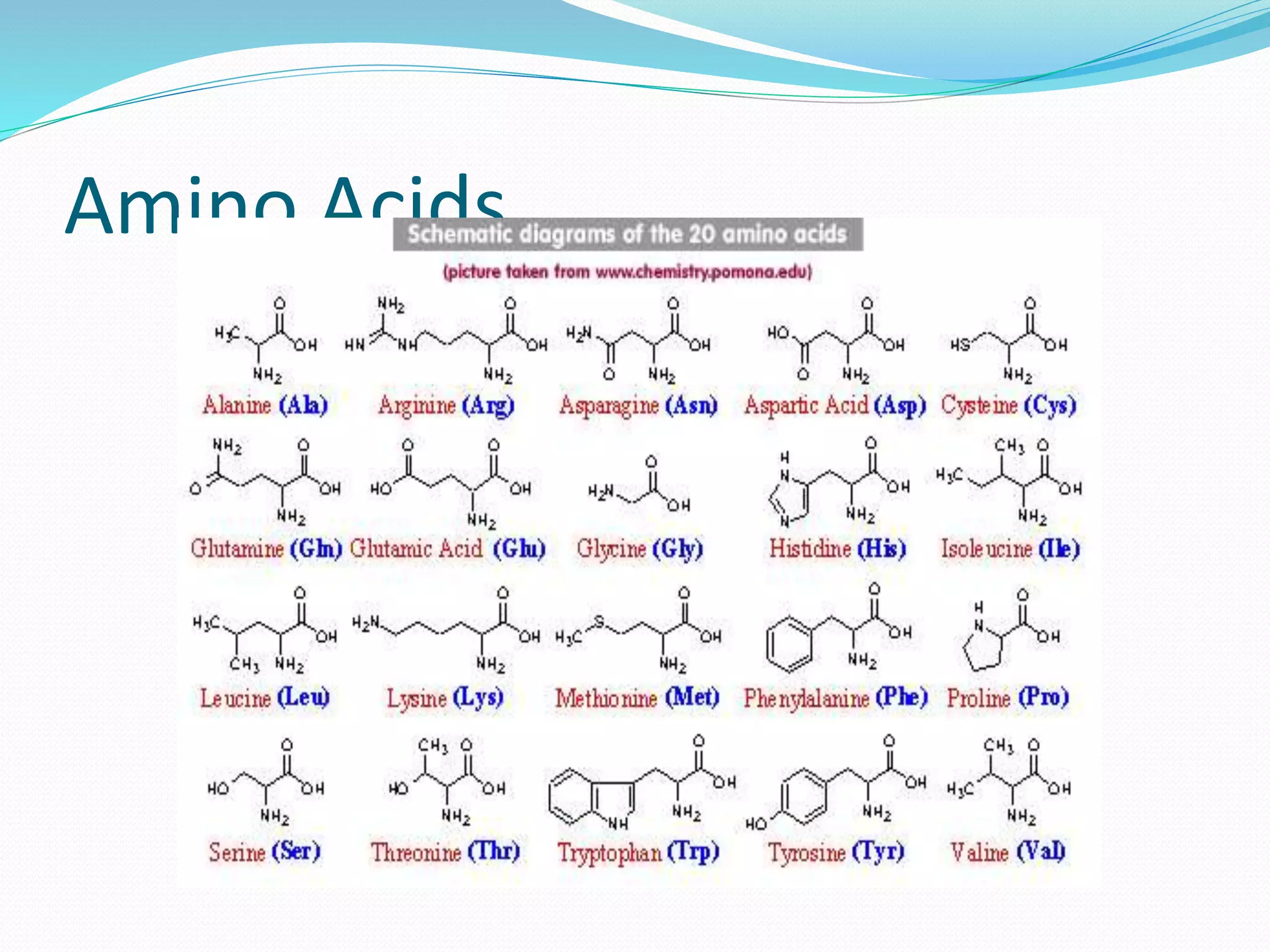
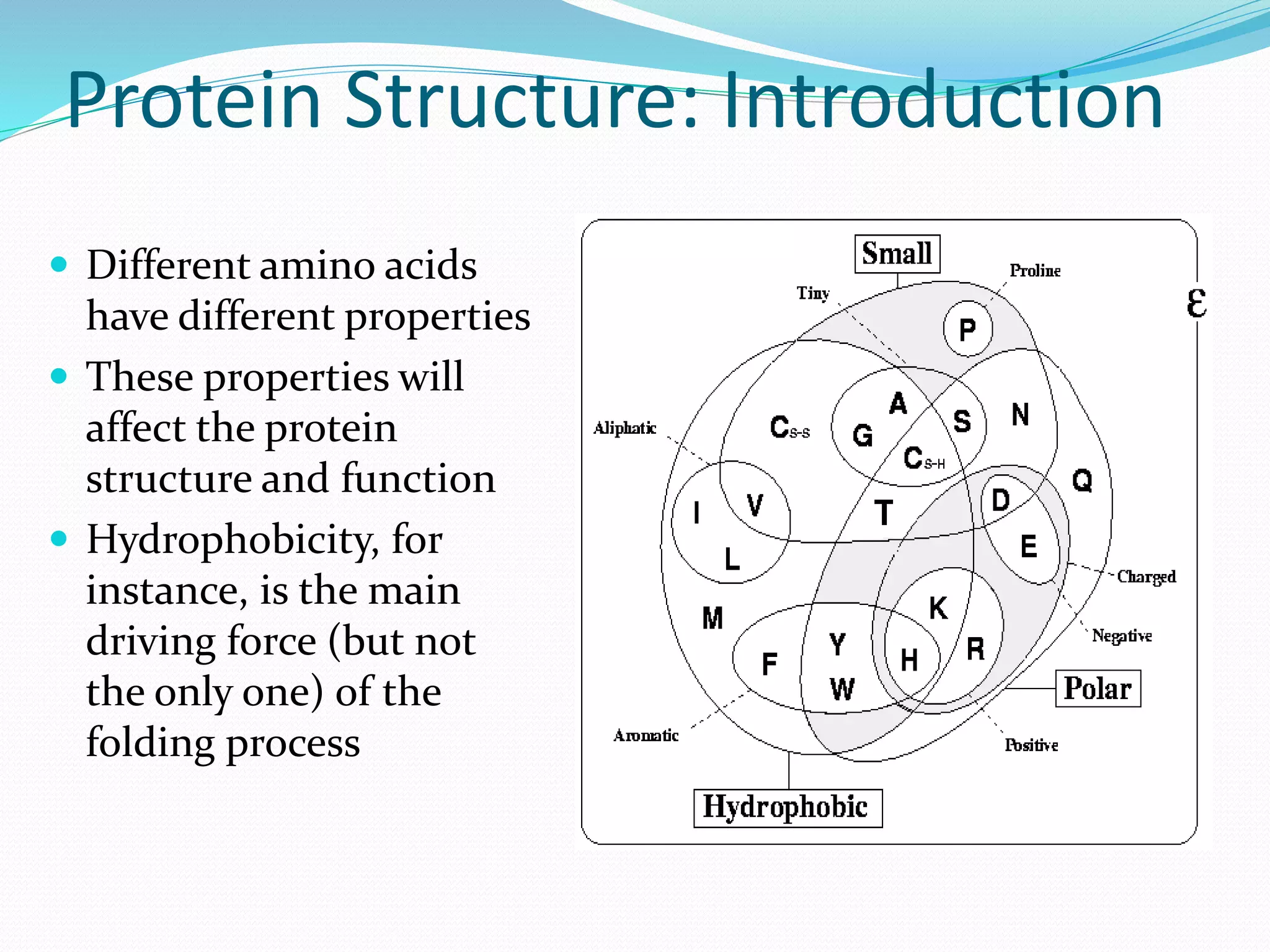
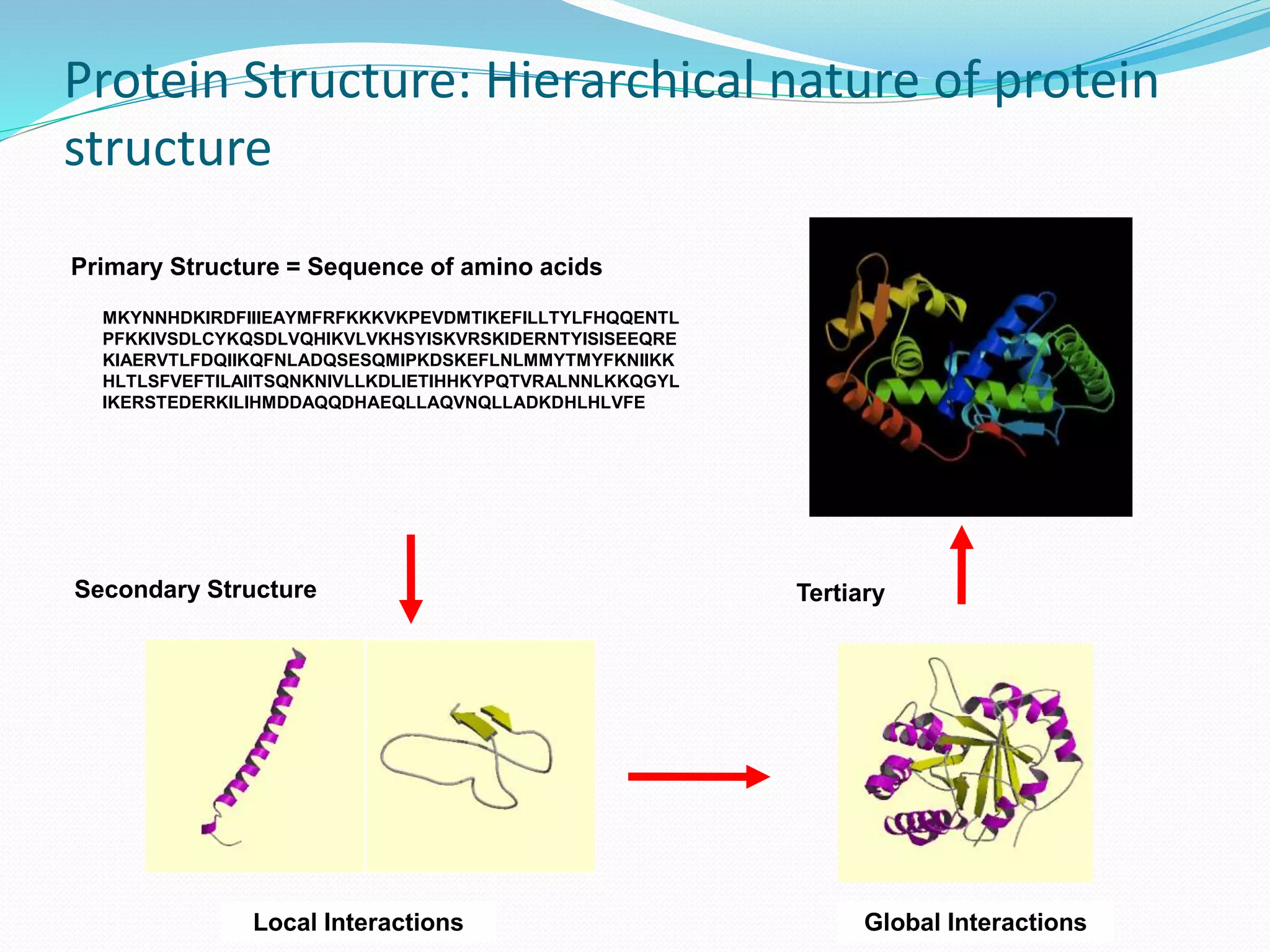
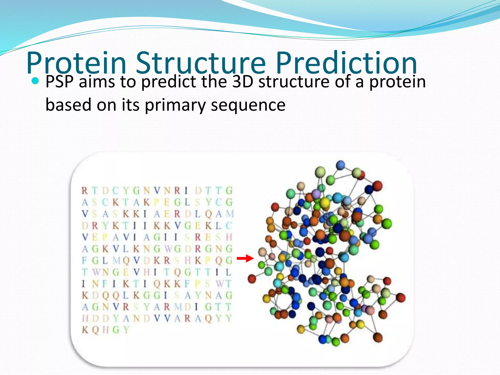
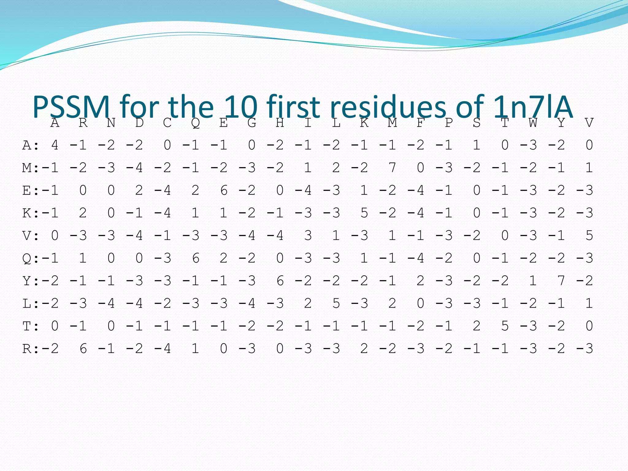
![Target for reduction: the primary sequence
The primary sequence of a protein is
an usual target for such simplification
It is composed of a quite high cardinality
alphabet of 20 symbols, which share
commonalities between them
One example of reduction widely used in
the community is the hydrophobic-polar
(HP) alphabet, reducing these 20 symbols
to just two
HP representation usually is too simple,
too much information is lost in the
reduction process [Stout et al., 06]
Can we automatically generate these
reduced alphabets and tailor them to
the specific problem at hand?](https://image.slidesharecdn.com/introduction-170331154845/75/Introduction-128-2048.jpg)
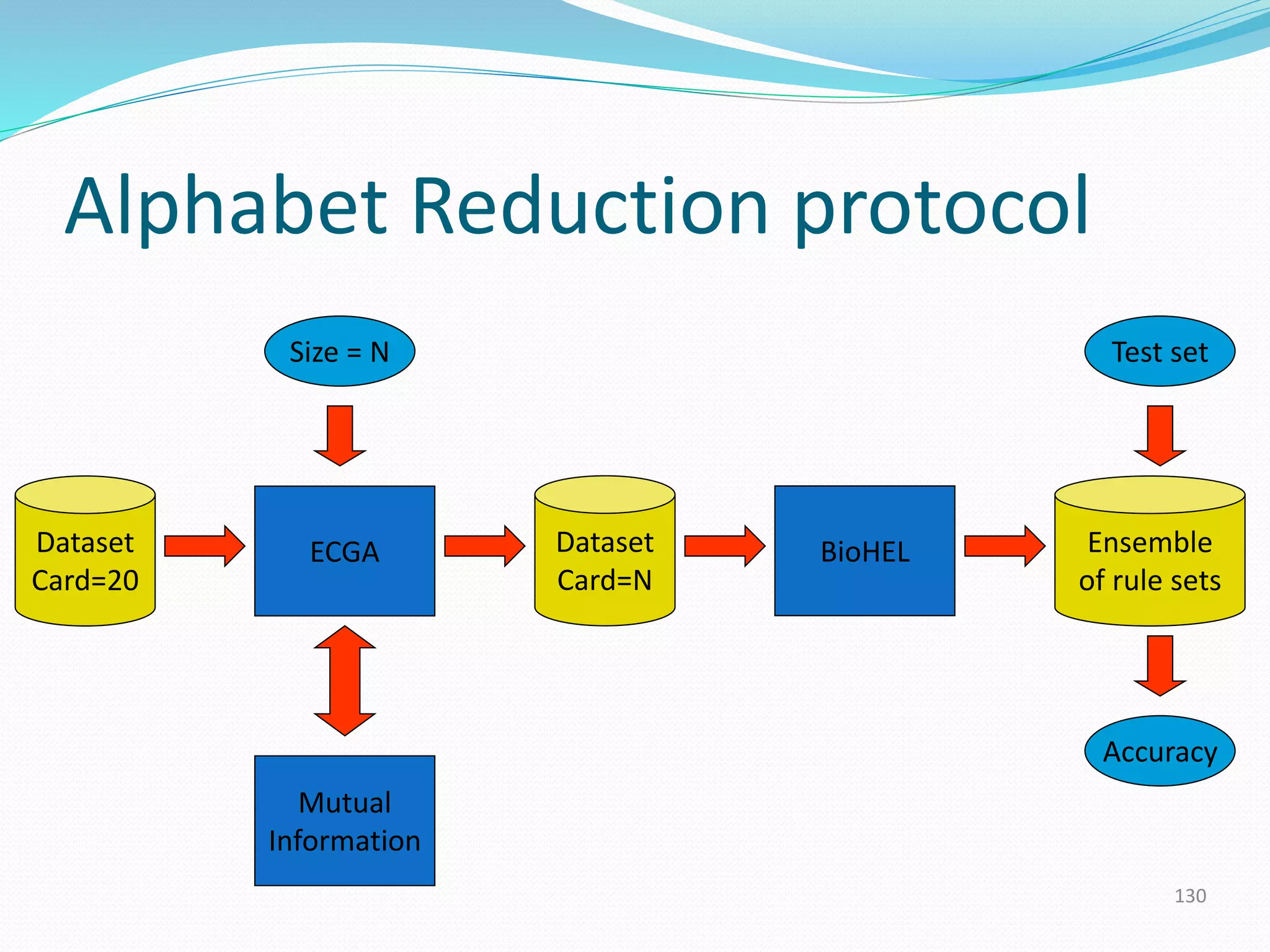
![Automated Alphabet Reduction
[Bacardit et al., 09]
• We will use an automated information theory-driven
method to optimize alphabet reduction policies for PSP
datasets
• An optimization algorithm will cluster the AA alphabet into
a predefined number of new letters
• Fitness function of optimization is based on the Mutual
Information (MI) metric. A metric that quantifies the
interrelationship between two discrete variables
– Aim is to find the reduced representation that maintains as much
relevant information as possible for the feature being predicted
• Afterwards we will feed the reduced dataset into a
learning method to verify if the reduction was proper](https://image.slidesharecdn.com/introduction-170331154845/75/Introduction-129-2048.jpg)
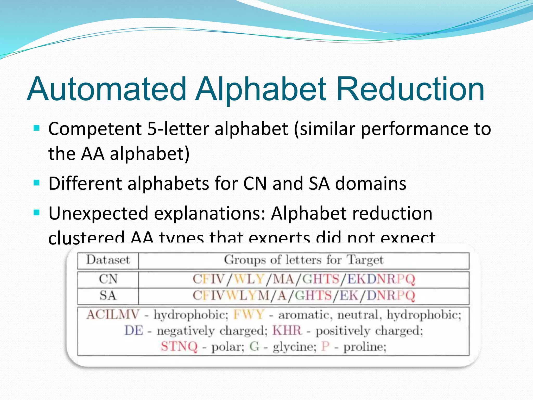
![Automated Alphabet Reduction
Our method produces better reduced alphabets than other
reduced alphabets from the literature and than other expert-
designed ones
Alphabets
from the
literature
Expert
designed
alphabets
Alphabet Letters CN acc. SA acc. Diff. Ref.
AA 20 74.0±0.6 70.7±0.4 --- ---
Our method 5 73.3±0.5 70.3±0.4 0.7/0.4 [Bacardit et al., 07]
WW5 6 73.1±0.7 69.6±0.4 0.9/1.1 [Wang & Wang, 99]
SR5 6 73.1±0.7 69.6±0.4 0.9/1.1 [Solis & Rackovsky, 00]
MU4 5 72.6±0.7 69.4±0.4 1.4/1.3 [Murphy et al., 00]
MM5 6 73.1±0.6 69.3±0.3 0.9/1.4 [Melo & Marti-Renom, 06]
HD1 7 72.9±0.6 69.3±0.4 1.1/1.4 [Bacardit et al., 07]
HD2 9 73.0±0.6 69.3±0.4 1.0/1.4 [Bacardit et al., 07]
HD3 11 73.2±0.6 69.9±0.4 0.8/0.8 [Bacardit et al., 07]](https://image.slidesharecdn.com/introduction-170331154845/75/Introduction-132-2048.jpg)
![Efficiency gains from the alphabet
reduction
We have extrapolated the reduced alphabet to the much
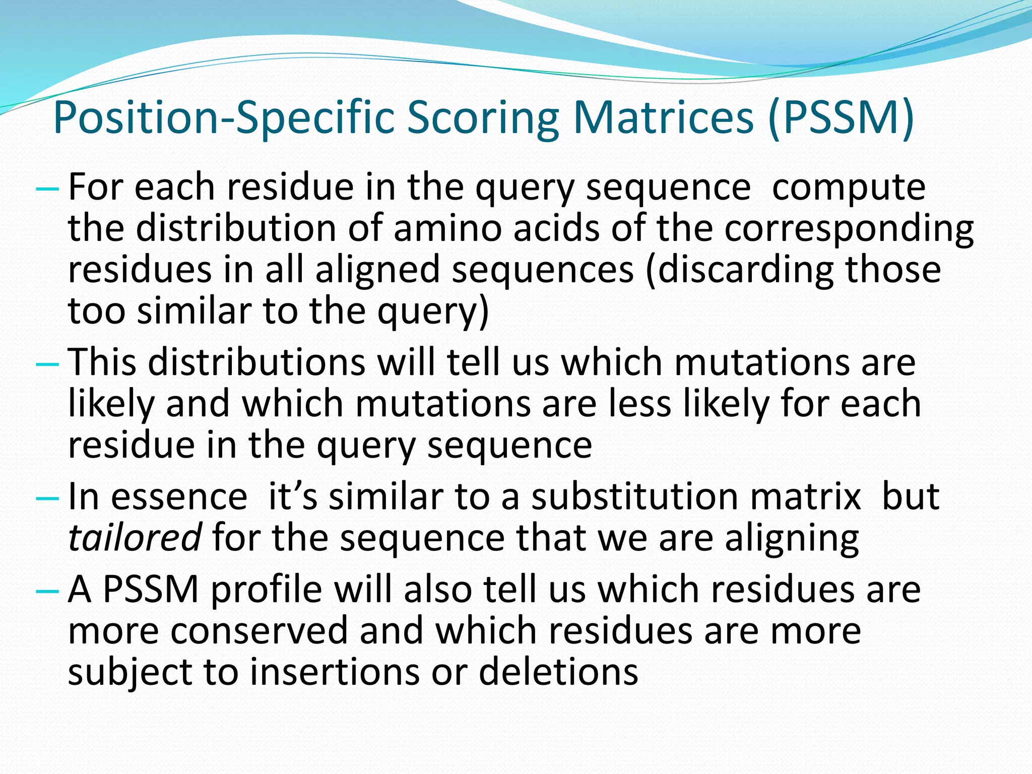
larger and richer Position-Specific Scoring Matrices (PSSM)
representation
Accuracy difference is still less than 1%
Obtained rule sets are simpler and training process is much
faster
Performance levels are similar to recent works in the literature
[Kinjo et al., 05][Dor and Zhou, 07]
Won the bronze medal of the 2007 Humies awards](https://image.slidesharecdn.com/introduction-170331154845/75/Introduction-133-2048.jpg)