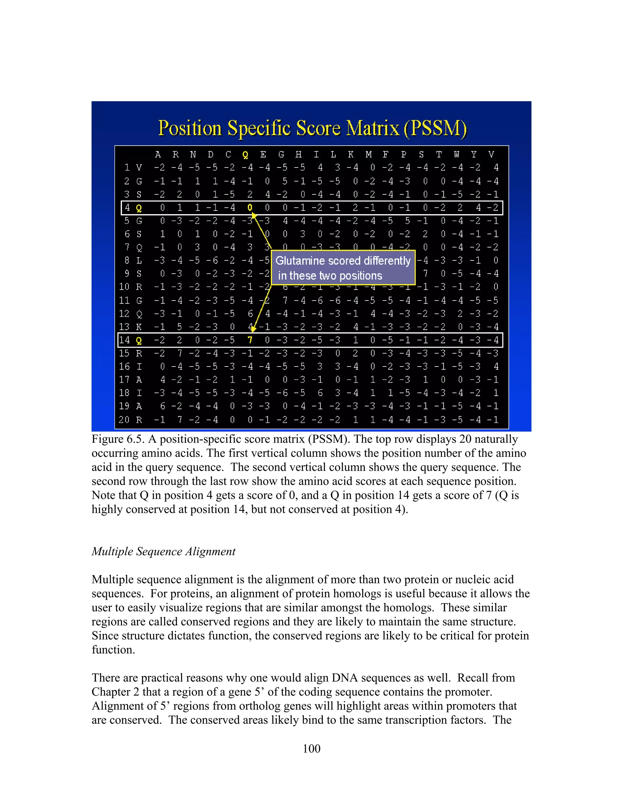
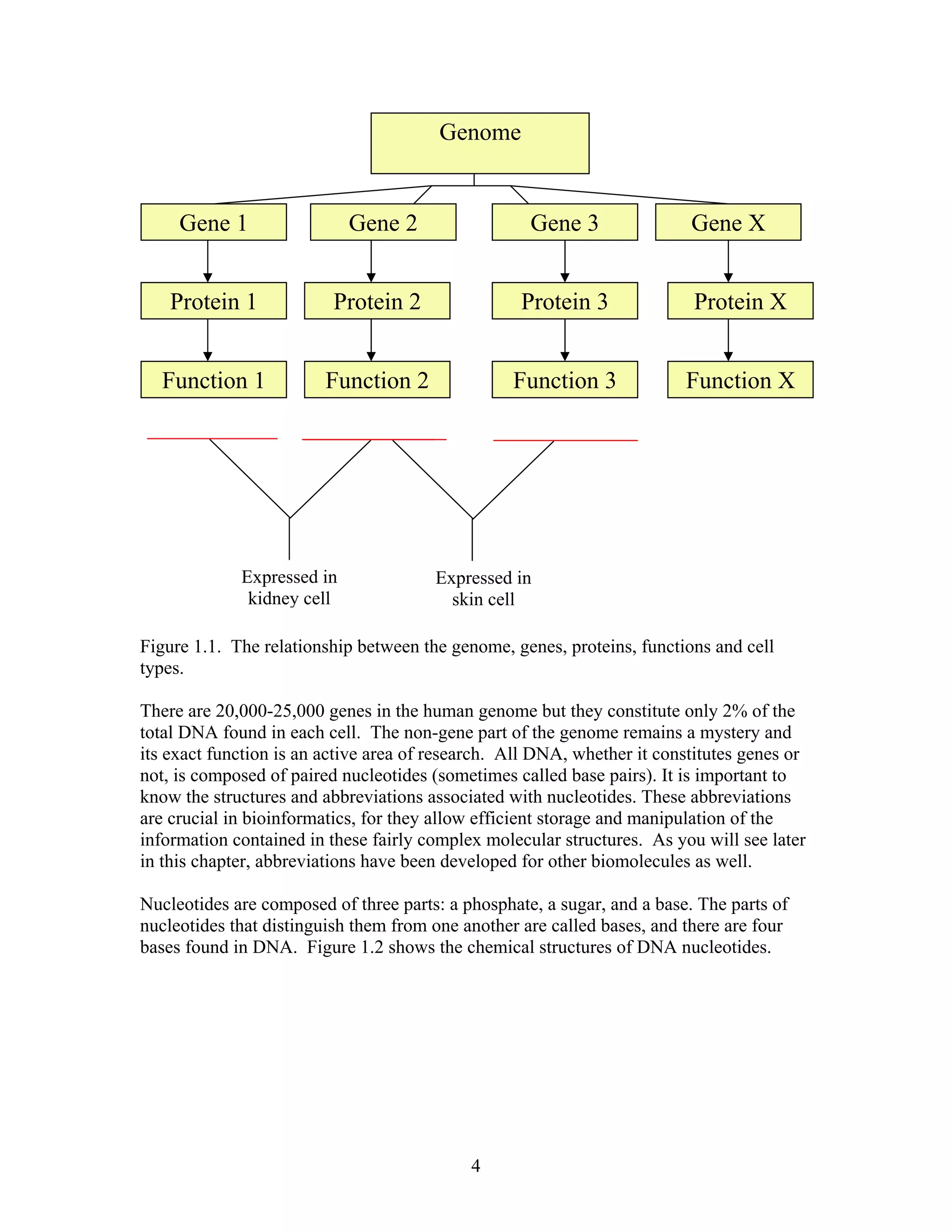
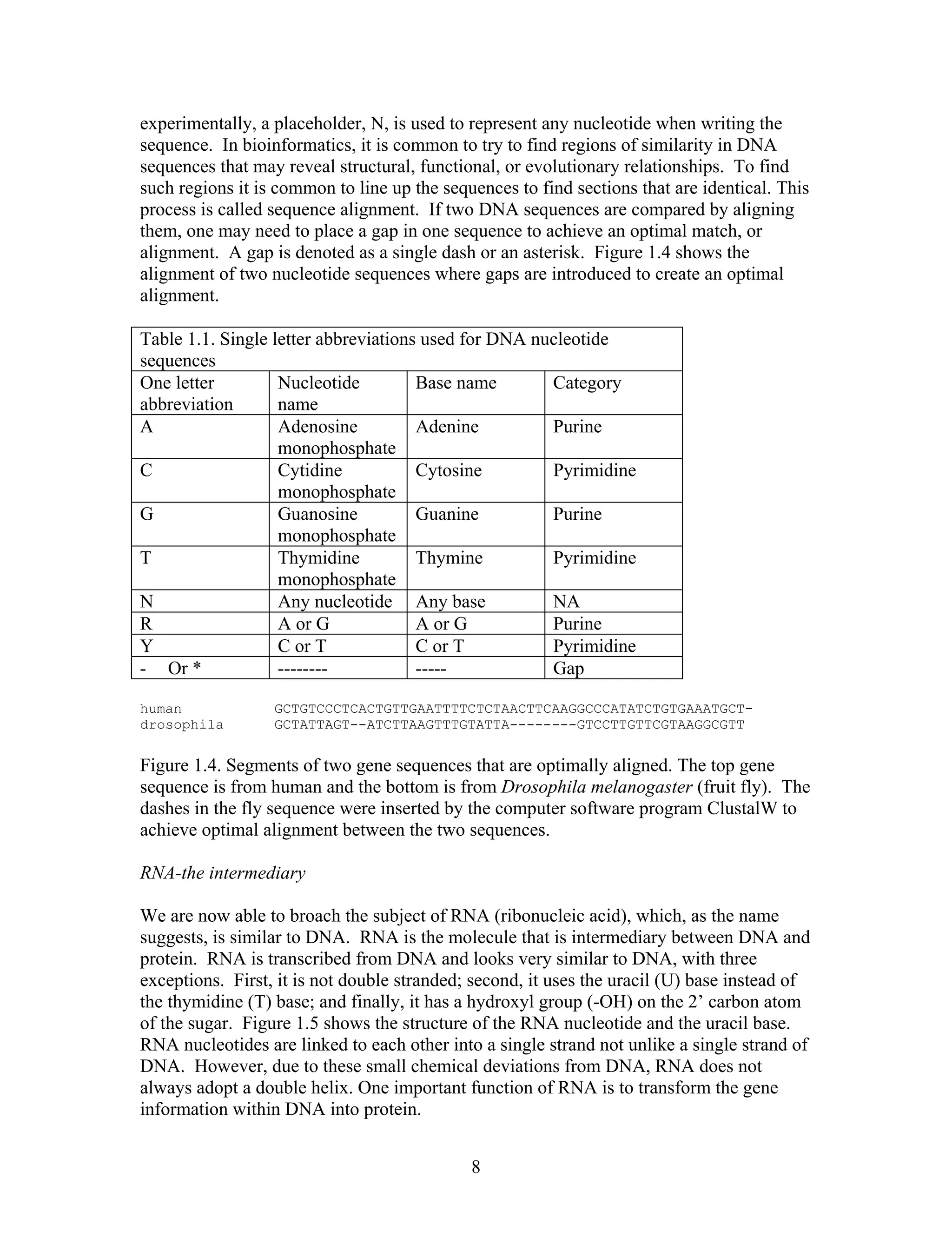
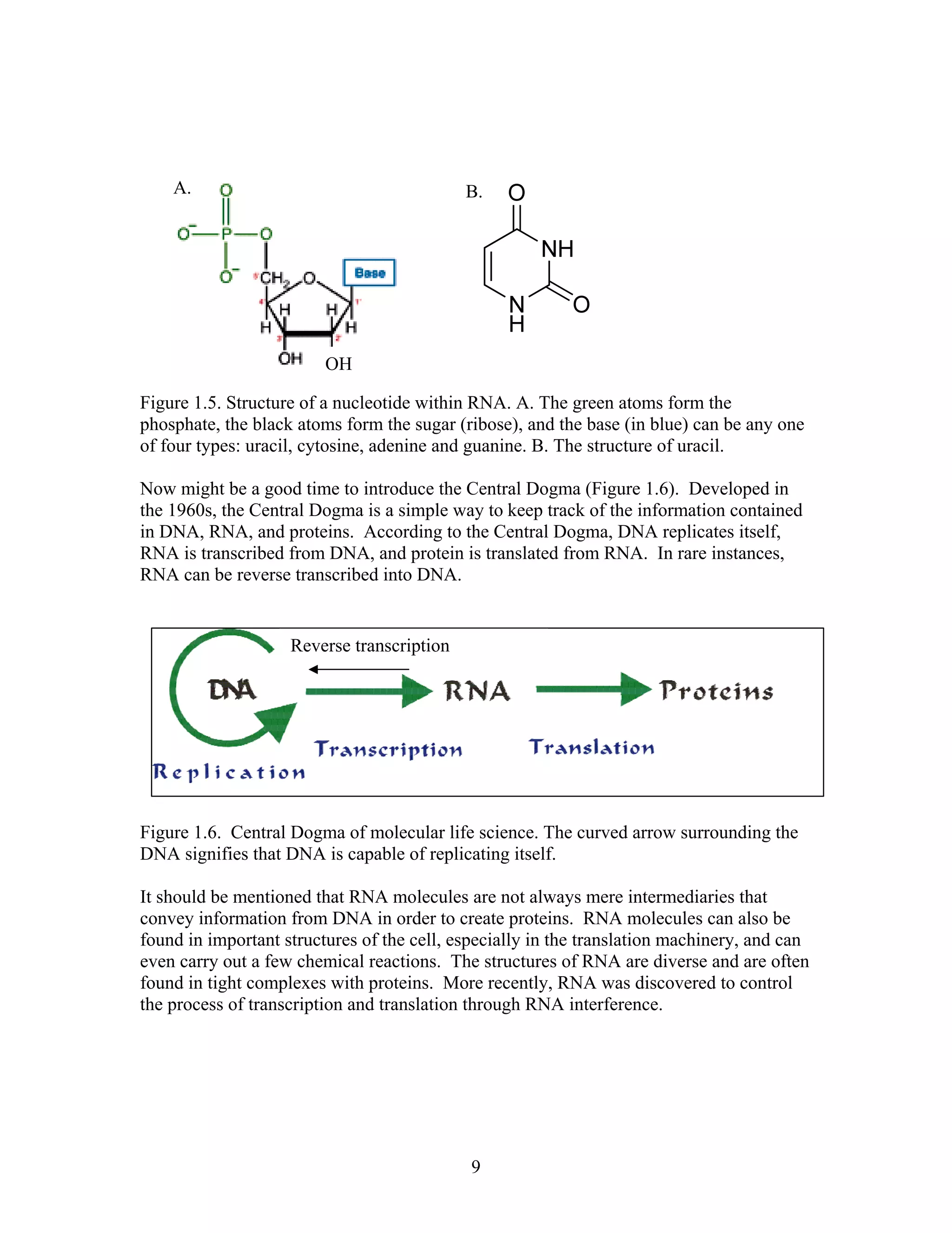
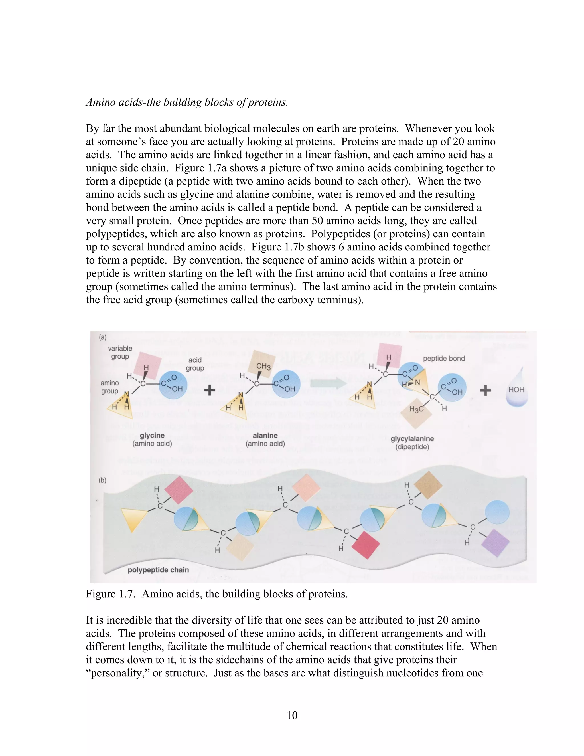
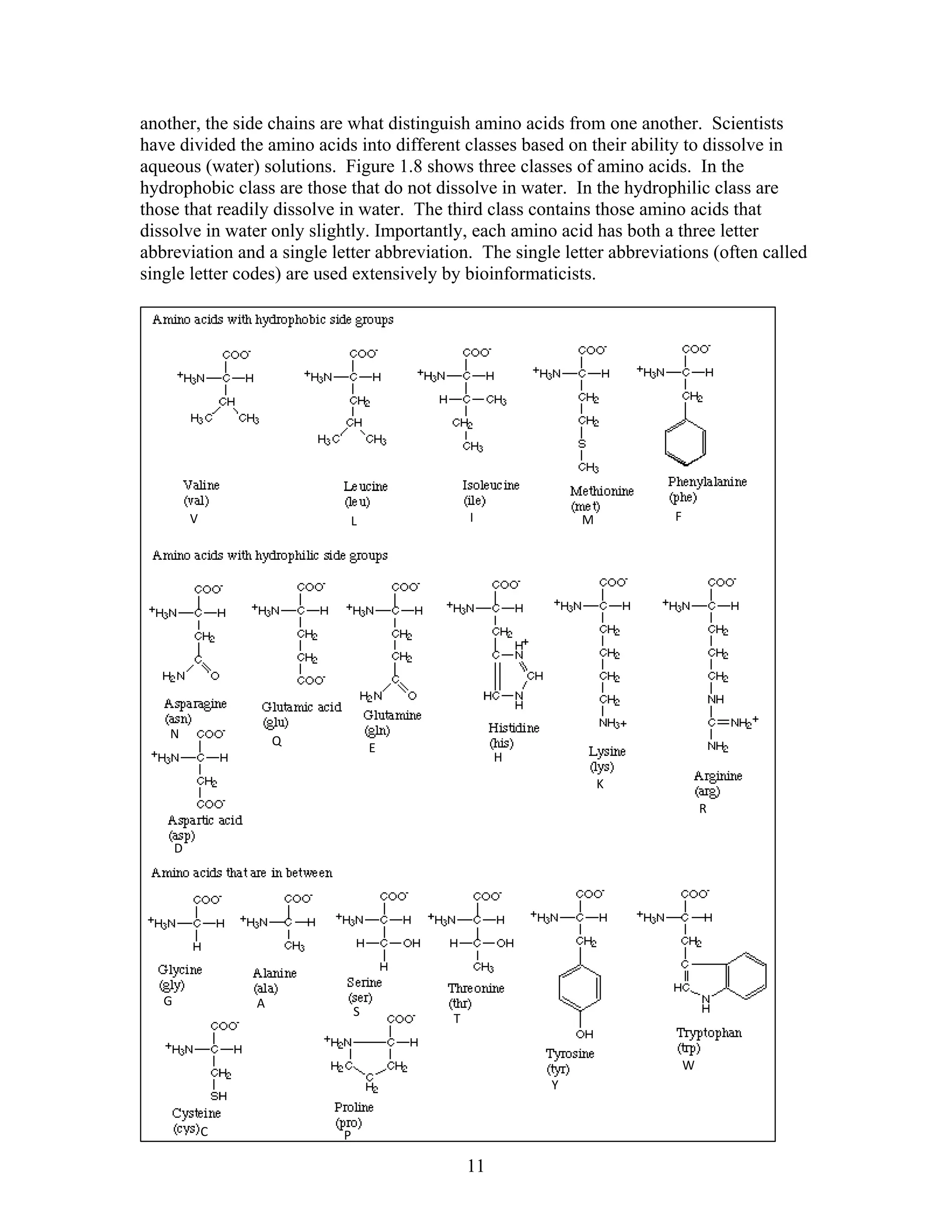
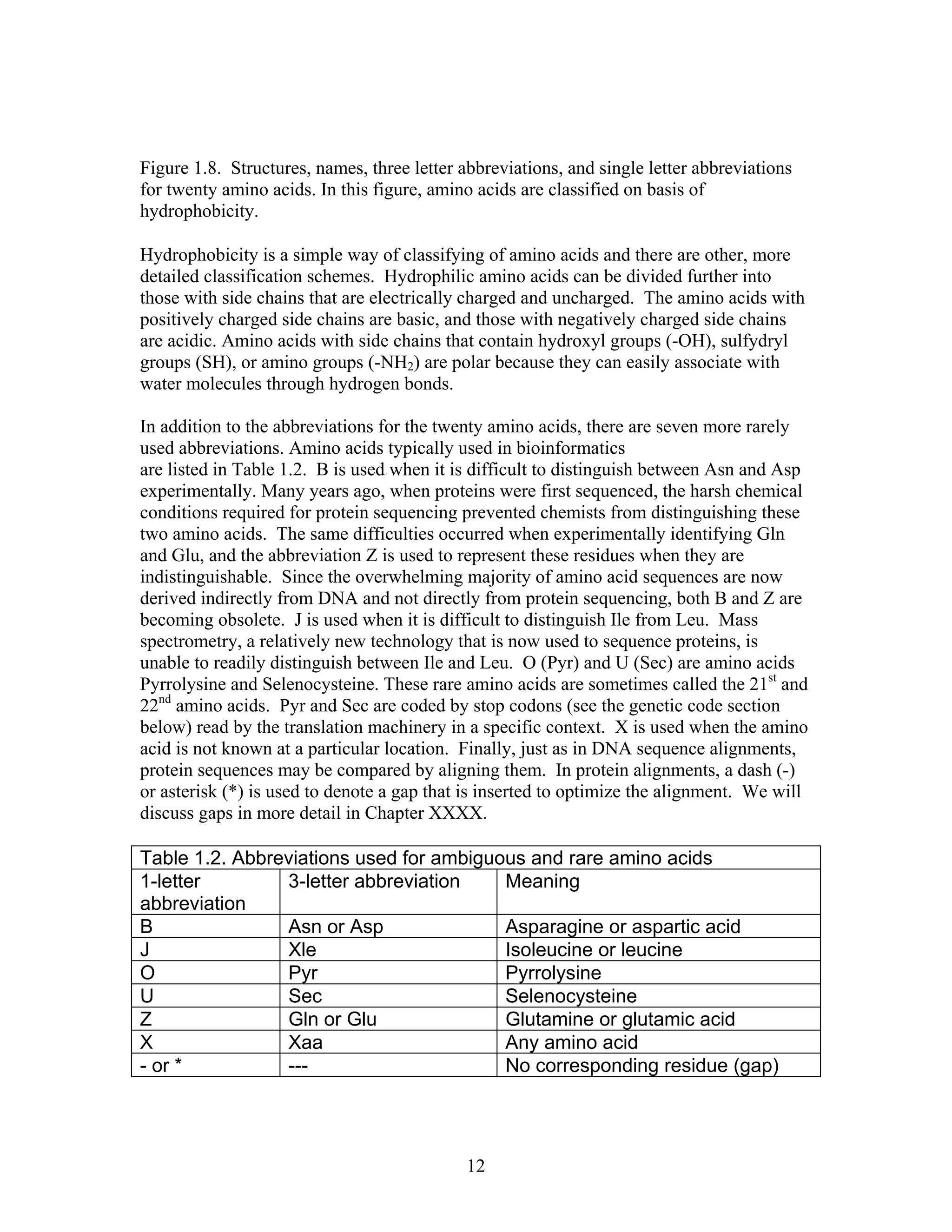
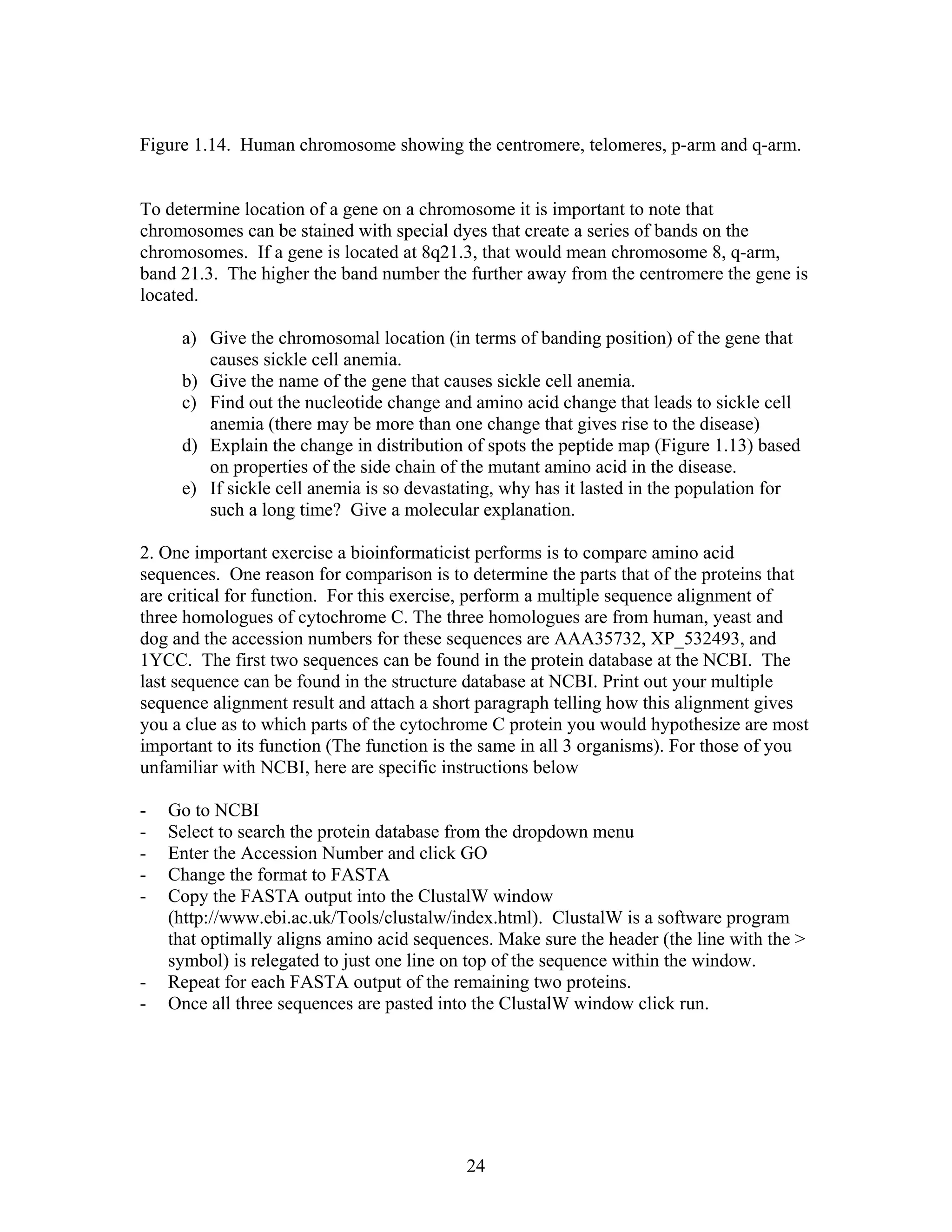
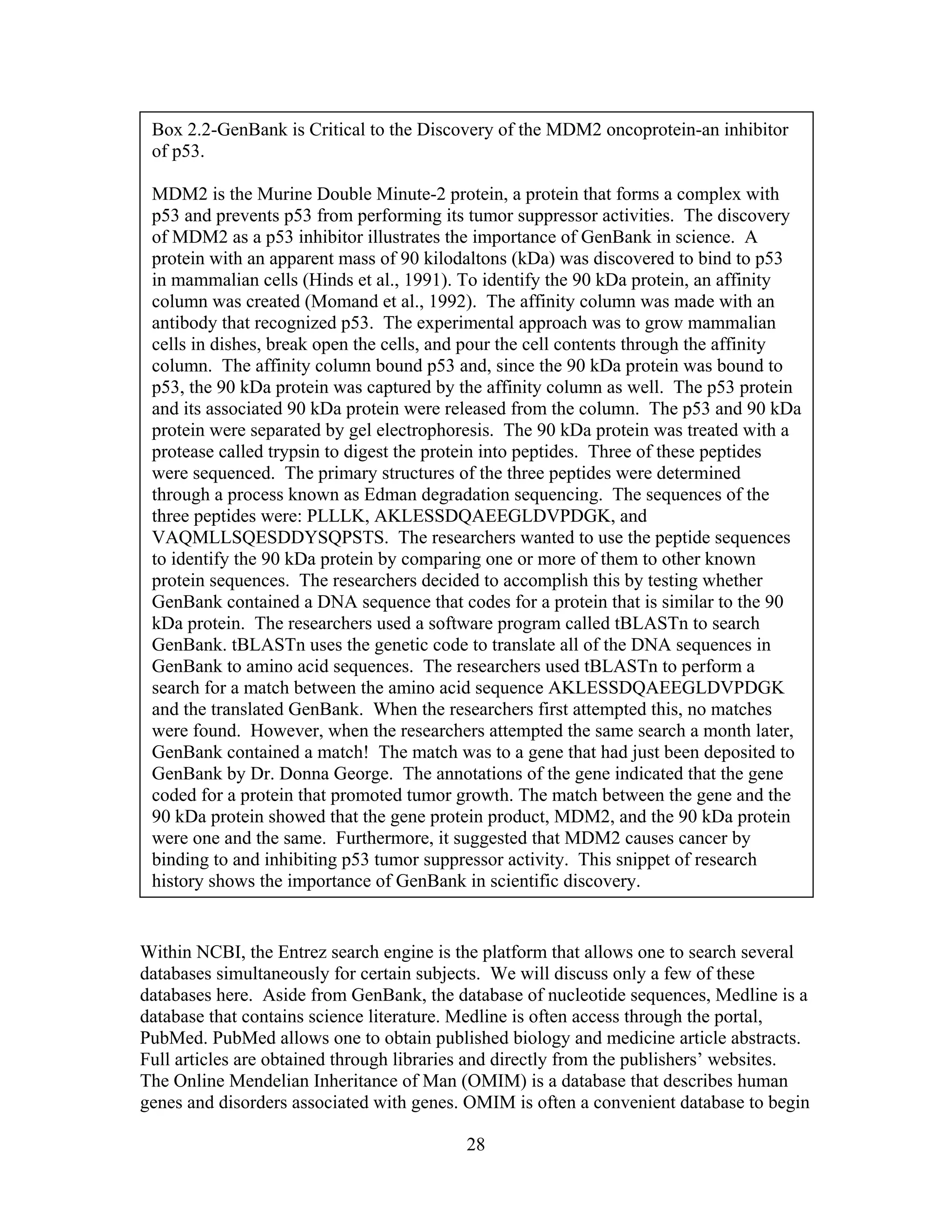
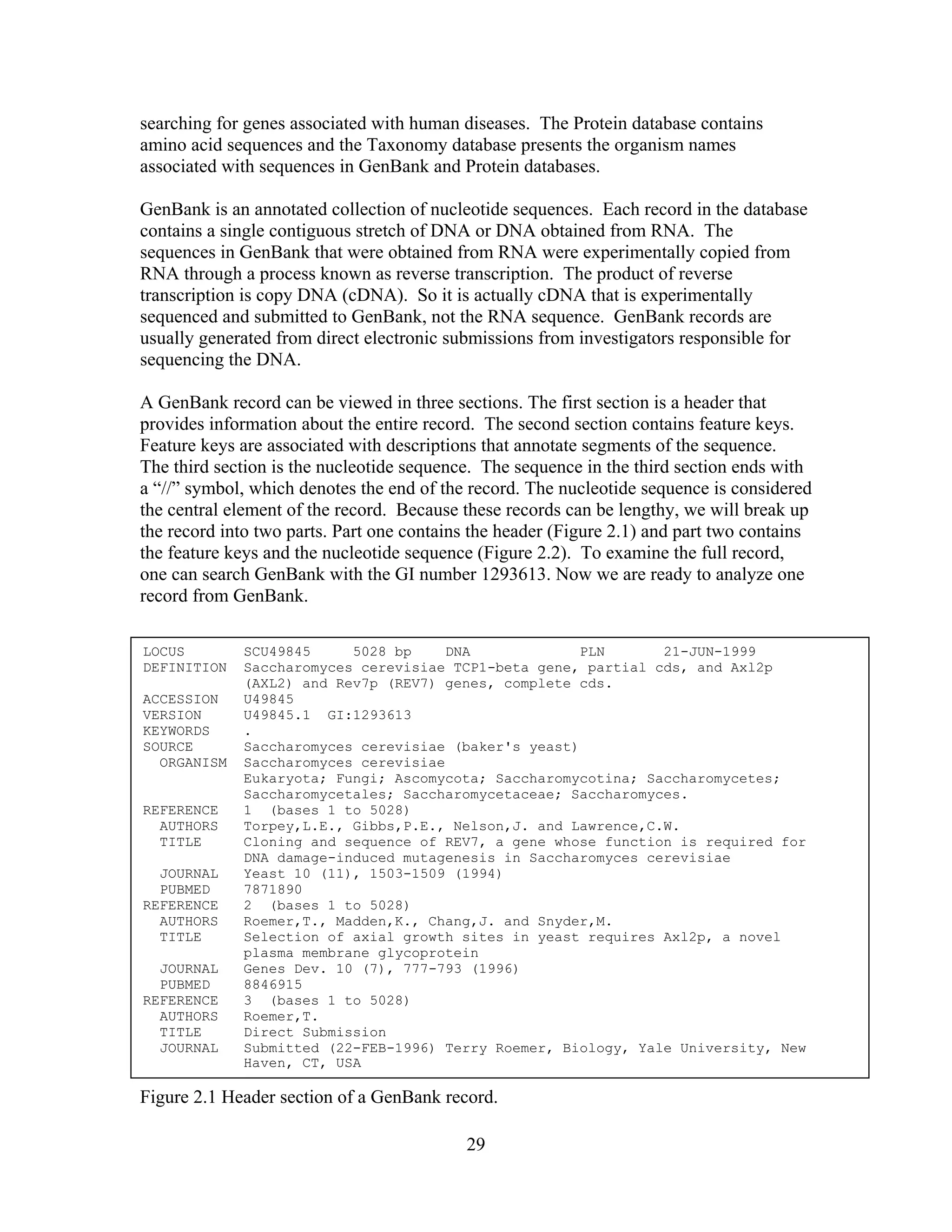
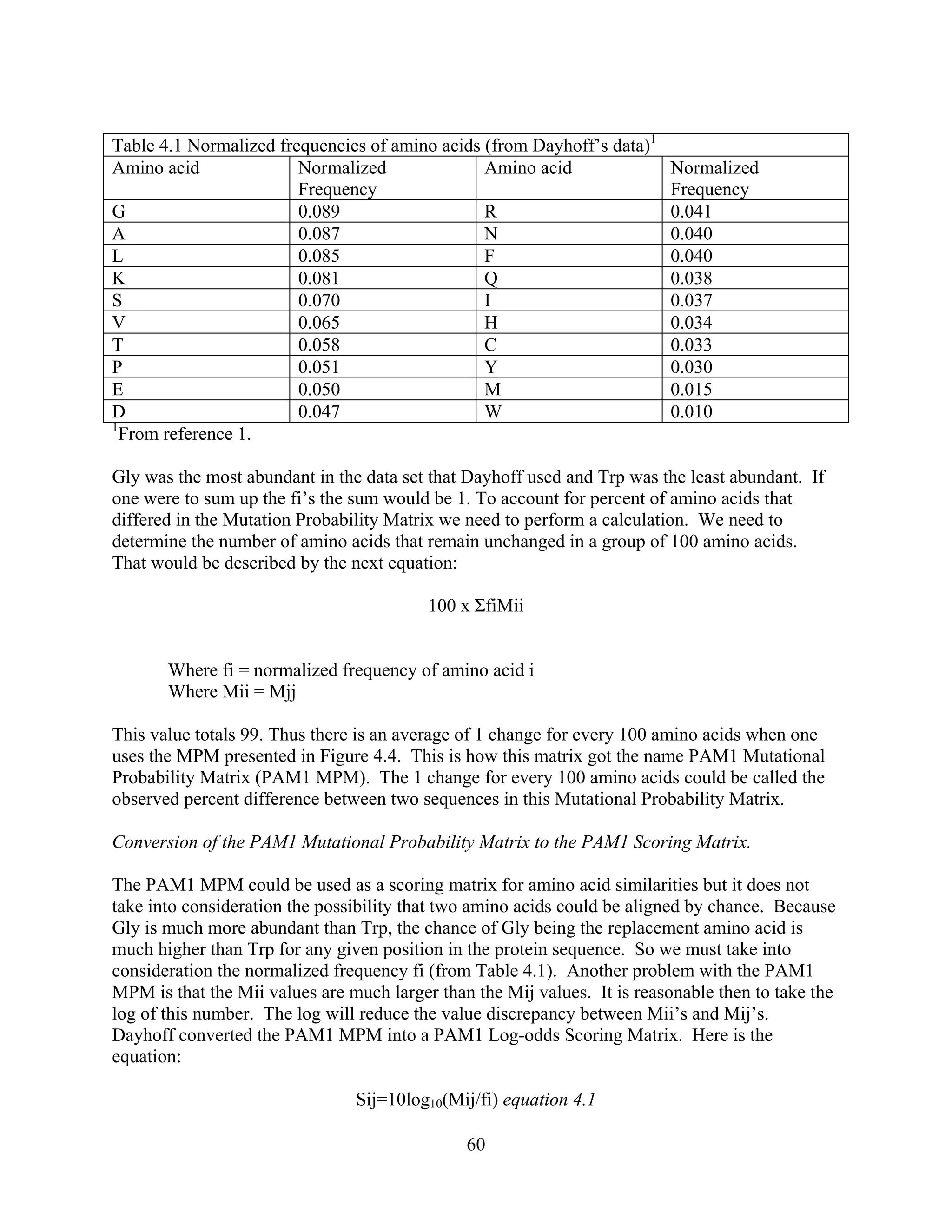
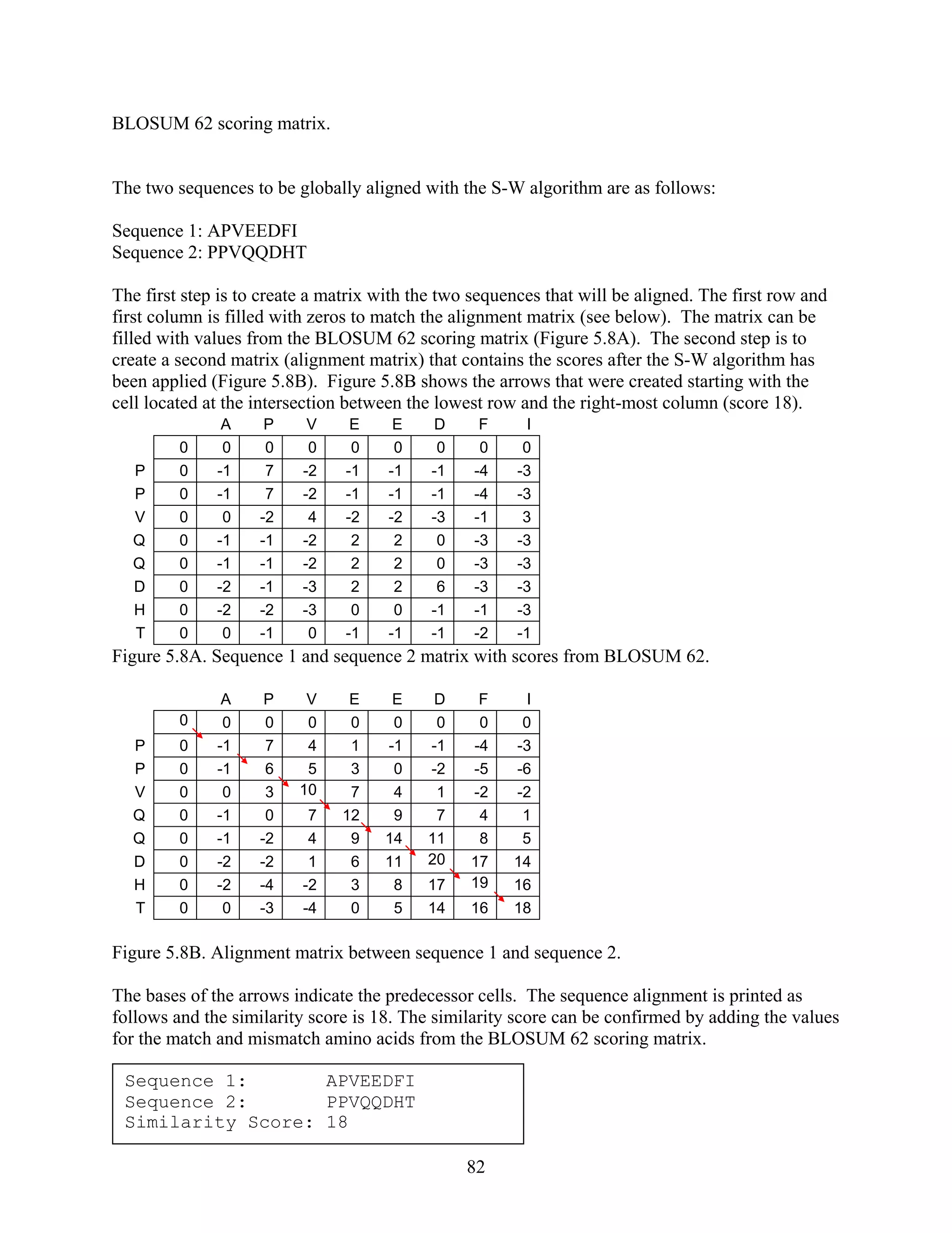
This document provides an introduction to bioinformatics. It begins by explaining that biology data is being collected rapidly and stored in databases, while software tools to analyze this data are also developing. Bioinformatics is defined as the research, development or application of computational tools and approaches for expanding the use of biological data. The document then reviews key molecular biology concepts like DNA, RNA, genes, proteins and the central dogma to provide context for bioinformatics. It distinguishes between bioinformatics users and developers, and notes that the field has expanded with genomic analysis.
![the gap opening penalty is higher than the gap extension penalty. The theory is that it would
require great evolutionary pressure to cause a one amino acid insertion or deletion. However,
once the “decision” has been made to create an insertion or deletion, the idea of adding more
amino acids to the insertion/deletion does not require more evolutionary pressure. Earlier in this
chapter we discussed scientific principles behind the derivation of the PAM and BLOSUM
scoring matrices. Generally there is less rigor in assigning values for gap opening and gap
extension penalties.
Aspects of the N-W Global Alignment system are used for multiple sequence alignment
programs. In multiple sequence alignment programs, many sequences are globally aligned
pairwise prior to compilation of the sequences. We will discuss multiple sequence alignment
programs in Chapter 6.
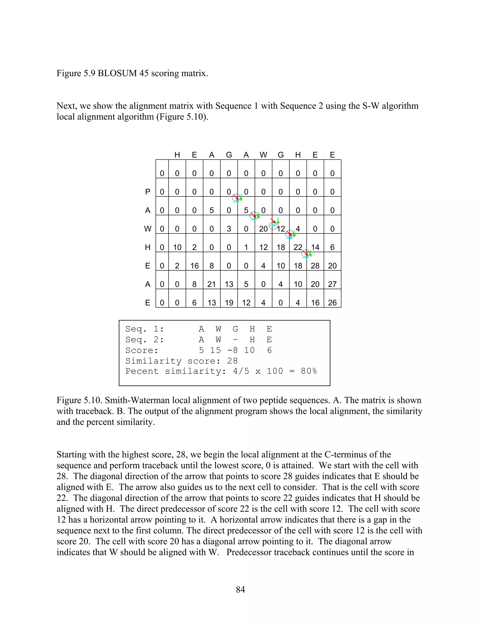
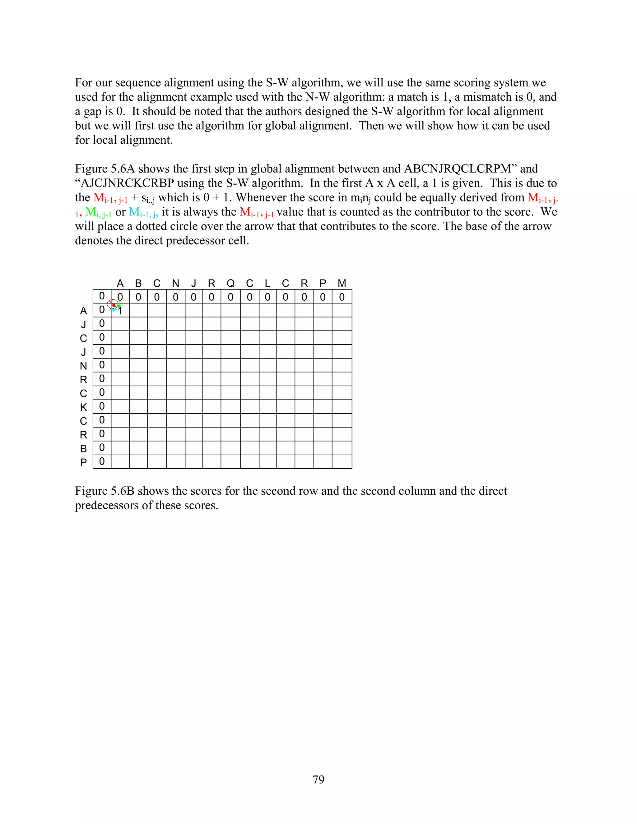
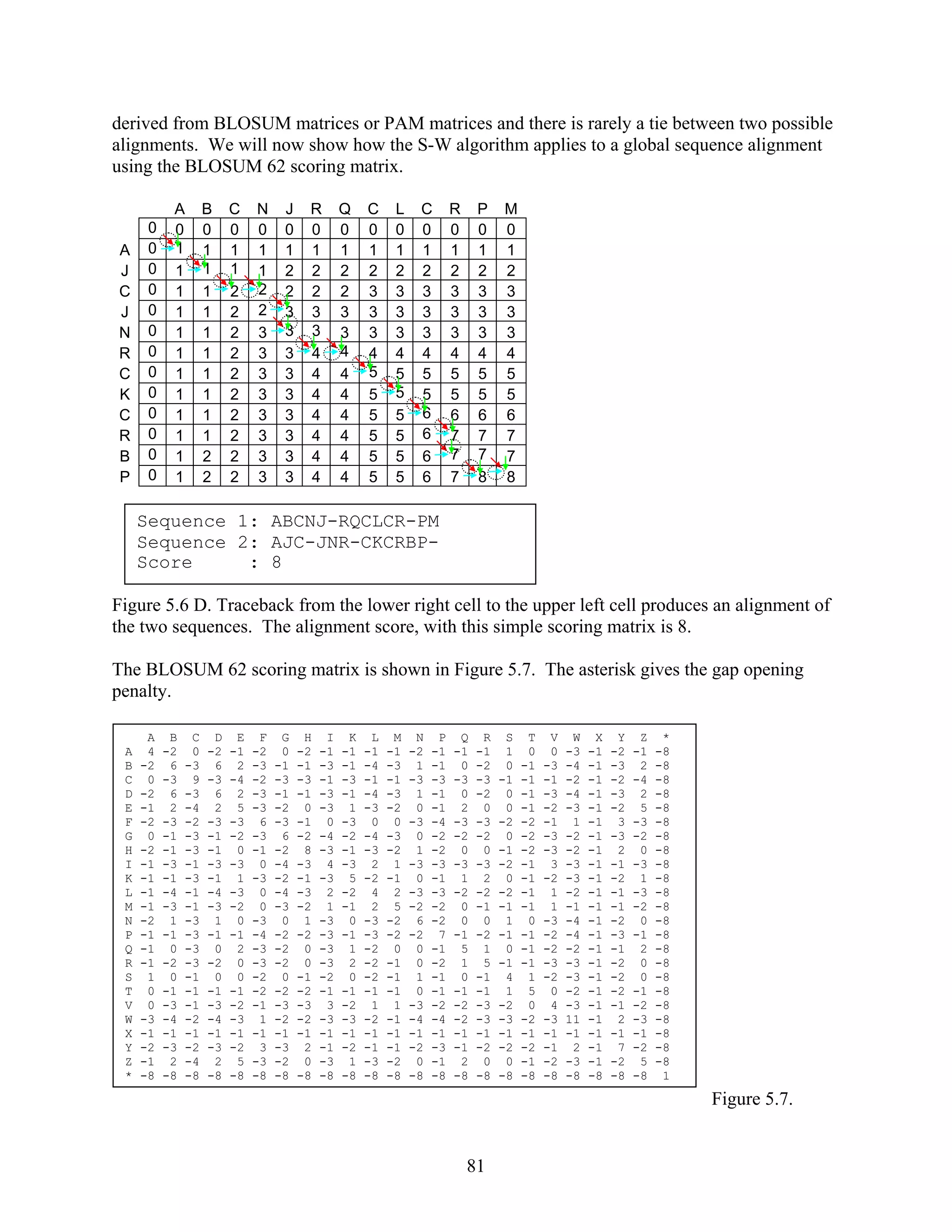
The Smith-Waterman Algorithm
The Smith-Waterman (S-W) algorithm can be used to find global or local alignments in
sequences (Smith and Waterman, 1981). Principles of the algorithm will be discussed here. We
will demonstrate how to use the S-W algorithm to perform a global alignment. This is useful
because we can compare the S-W algorithm to the N-W algorithm. Both algorithms give a high
score of 8 for sequences shown in Figure 5.4. Then we will use then use the S-W algorithm to
show how it can be used to detect local alignments.
Similar to the N-W algorithm, the S-W algorithm uses an initialization step, a matrix fill step,
and a trace-back step. When using the S-W algorithm let’s denote the number of letters in
sequence 1 as m and the number of letters in sequence 2 as n. A matrix is created with m + 1
columns and n + 1 rows. In the first step, zeros are placed in the m - 1 column and n - 1 row.
We define the location of a particular cell as minj. Next, a scoring system is created where Mi,j is
the maximum score in minj. The maximum score is always placed into each cell of the matrix.
The formal definition of Mi,j is:
Mi,,j = MAXIMUM [
Mi-1, j-1 + si,,j (match or mismatch value),
Mi, j-1 + w (gap in sequence #1),
Mi-1, j + w (gap in sequence #2)]
Where Mi-1, j-1 is the score in the cell diagonally juxtaposed to minj. The i-1, j-1 cell is up and to
the left of mi,nj.
Where si,j is the value for the match or mismatch in the minj.
Where Mi, j-1 is the score in the cell above minj.
Where w is the value for the gap penalty.
Where Mi-1, j is the score in the cell to the left of minj.
78](https://image.slidesharecdn.com/bioinformaticsmanual-170311105329/75/Bioinformatics-manual-78-2048.jpg)
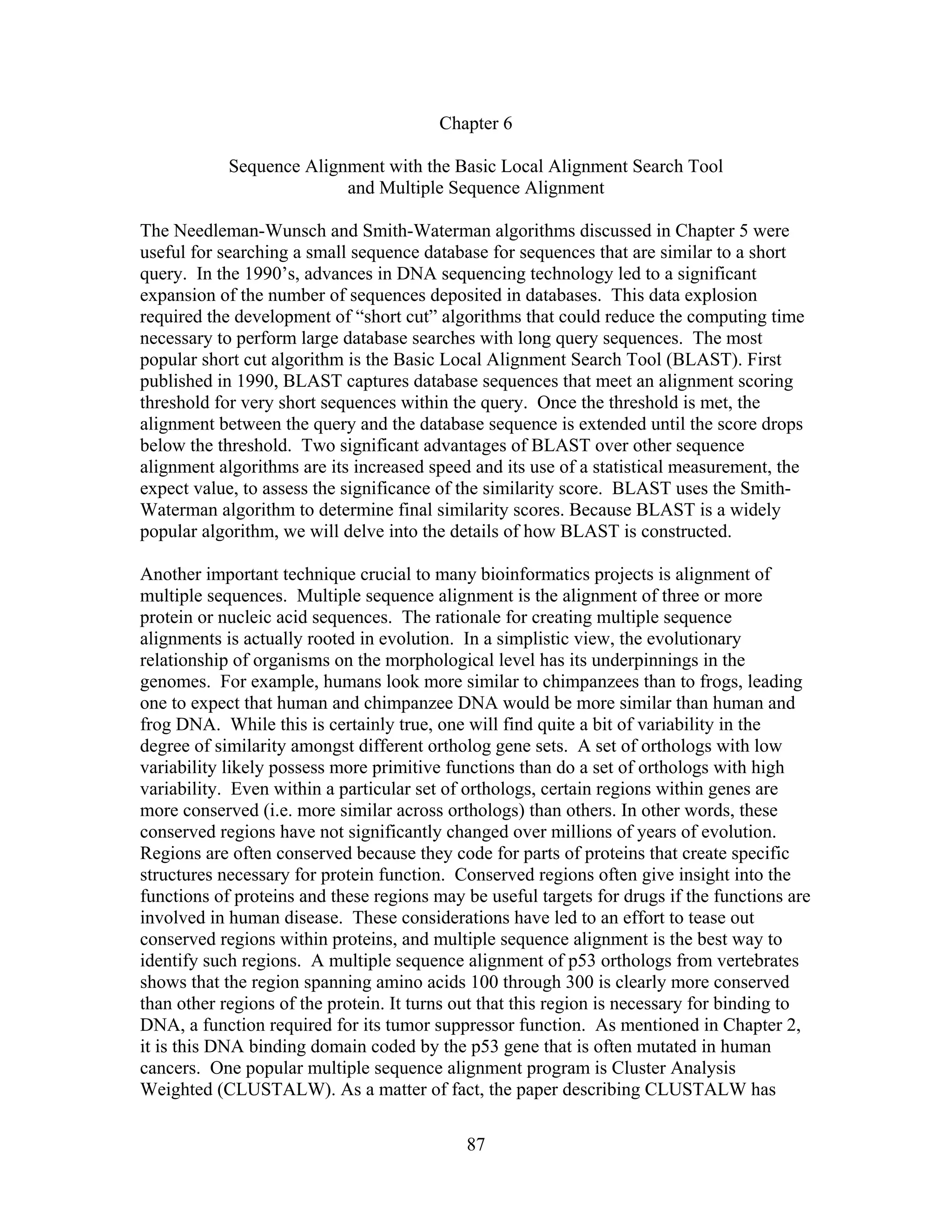
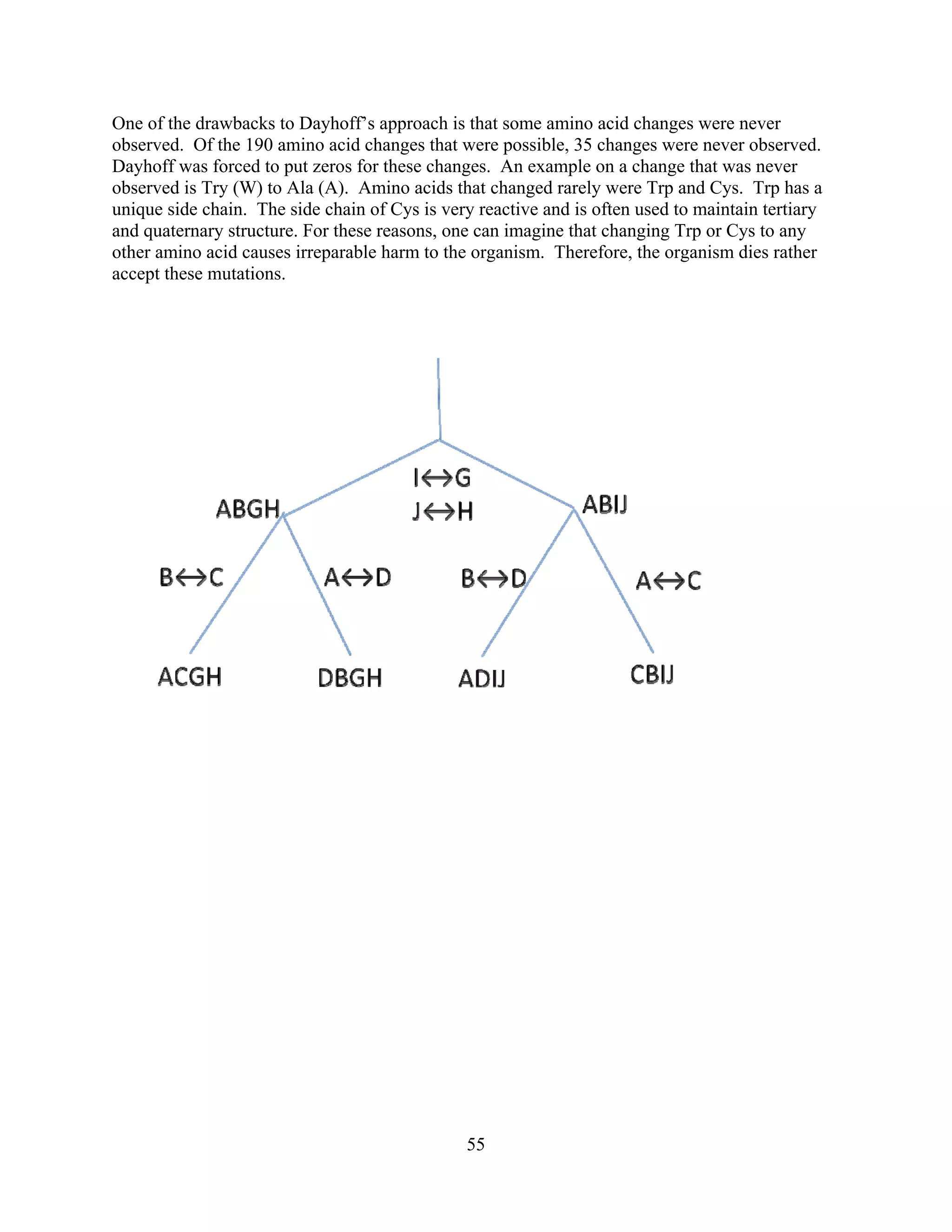
![For local alignment, a modification of the S-W global alignment algorithm is used.
value),
p in sequence #2),
0]
ith
If
or
is placed in Sequence 2 (the sequence displayed next to the first column of the
atrix).
aterman local alignment algorithm will be used to compare the following
quences:
EE
equence 2: PAWHEAE
fault gap penalty.
Mi,,j = MAXIMUM [
Mi-1, j-1 + si,,j (match or mismatch
Mi, j-1 + w (gap in sequence #1),
Mi-1, j + w (ga
The modification is that no score in the alignment matrix will be less than zero. Once the
alignment matrix is filled, the algorithm searches each cell for the highest score. Starting w
the cell with highest score, the algorithm traces back until a cell with zero is reached. The
algorithm returns to the user the amino acids aligned in the traceback and the similarity score.
the traceback contains a vertical predecessor cell, a gap is placed in Sequence 1 (the sequence
displayed above the top row of the matrix). If the traceback contains a horizontal predecess
cell, a gap
m
The Smith-W
se
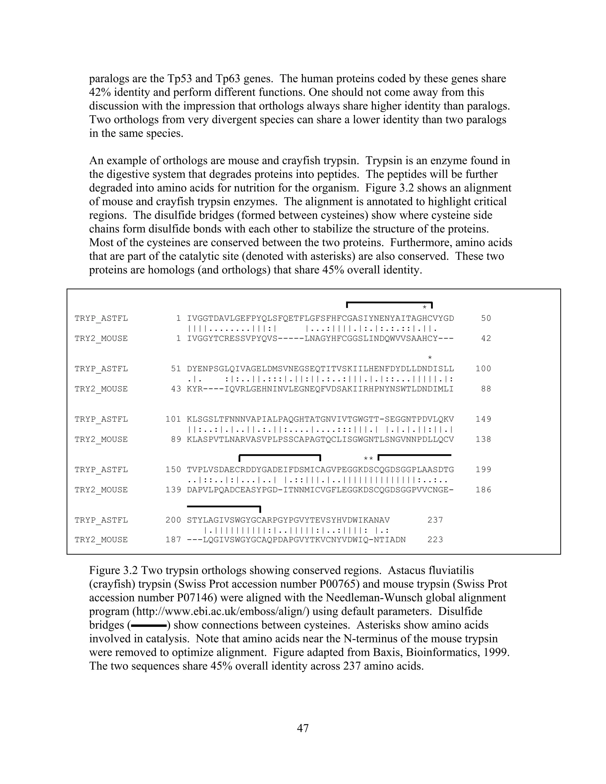
Sequence 1: HEAGAWGH
S
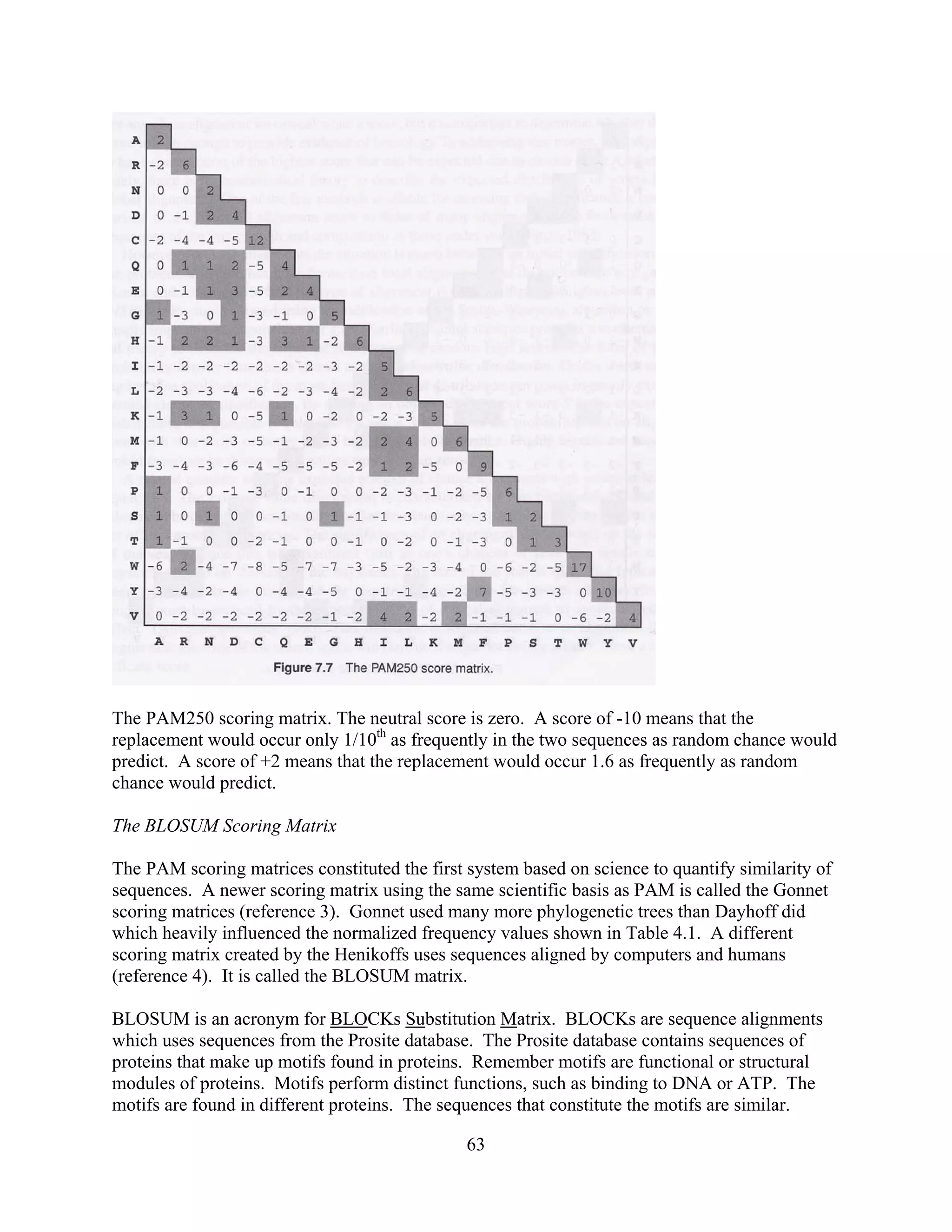
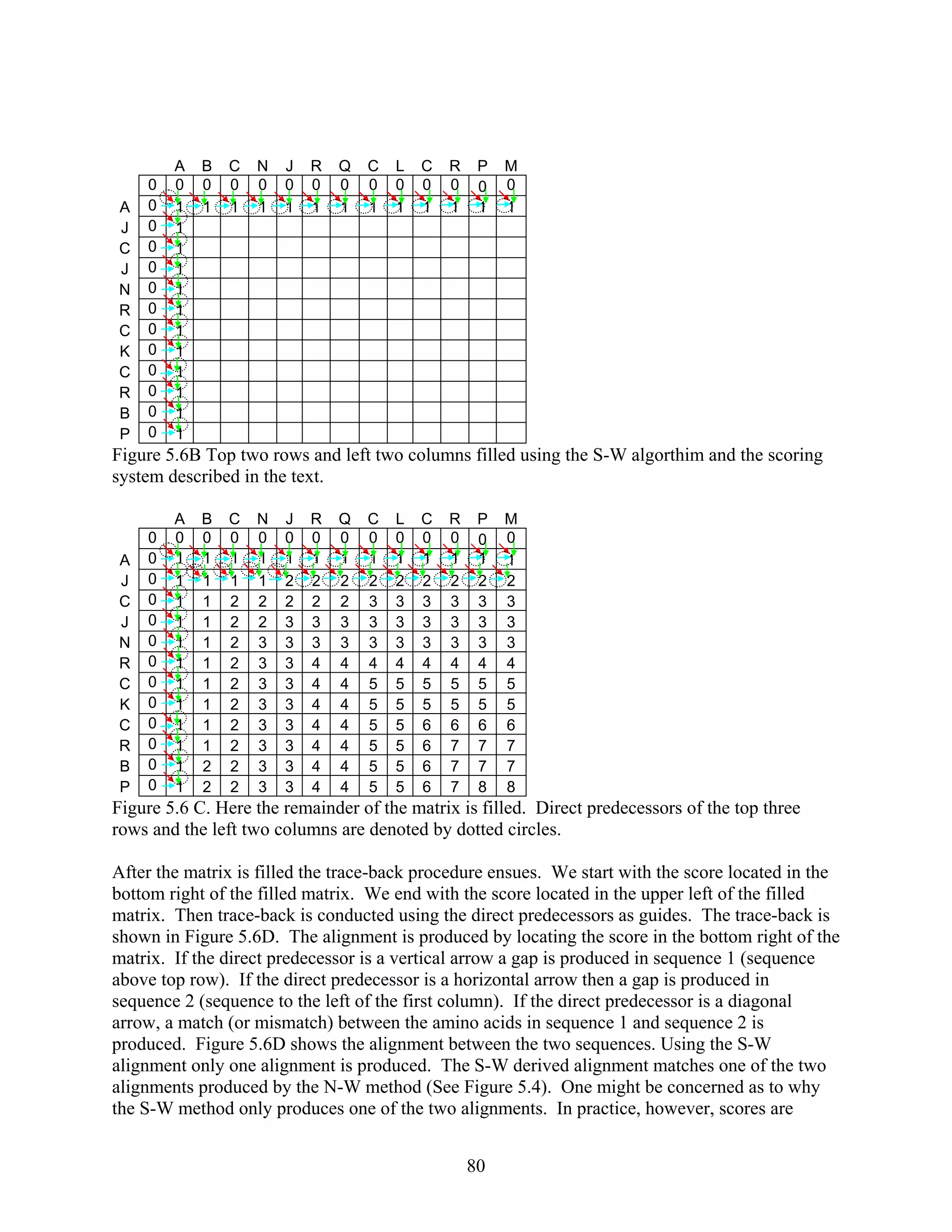
For this alignment, we will use the BLOSUM 45 scoring matrix (Figure 5.9) with one small
change. The change is that we will use a gap penalty of -8 instead of the -5 de
A B C D E F G H I K L M N P Q R S T V W X Y Z *
A 5 -1 -1 -2 -1 -2 0 -2 -1 -1 -1 -1 -1 -1 -1 -2 1 0 0 -2 0 -2 -1 -5
B -1 4 -2 5 1 -3 -1 0 -3 0 -3 -2 4 -2 0 -1 0 0 -3 -4 -1 -2 2 -5
C -1 -2 12 -3 -3 -2 -3 -3 -3 -3 -2 -2 -2 -4 -3 -3 -1 -1 -1 -5 -2 -3 -3 -5
D -2 5 -3 7 2 -4 -1 0 -4 0 -3 -3 2 -1 0 -1 0 -1 -3 -4 -1 -2 1 -5
E -1 1 -3 2 6 -3 -2 0 -3 1 -2 -2 0 0 2 0 0 -1 -3 -3 -1 -2 4 -5
F -2 -3 -2 -4 -3 8 -3 -2 0 -3 1 0 -2 -3 -4 -2 -2 -1 0 1 -1 3 -3 -5
G 0 -1 -3 -1 -2 -3 7 -2 -4 -2 -3 -2 0 -2 -2 -2 0 -2 -3 -2 -1 -3 -2 -5
H -2 0 -3 0 0 -2 -2 10 -3 -1 -2 0 1 -2 1 0 -1 -2 -3 -3 -1 2 0 -5
I -1 -3 -3 -4 -3 0 -4 -3 5 -3 2 2 -2 -2 -2 -3 -2 -1 3 -2 -1 0 -3 -5
K -1 0 -3 0 1 -3 -2 -1 -3 5 -3 -1 0 -1 1 3 -1 -1 -2 -2 -1 -1 1 -5
L -1 -3 -2 -3 -2 1 -3 -2 2 -3 5 2 -3 -3 -2 -2 -3 -1 1 -2 -1 0 -2 -5
M -1 -2 -2 -3 -2 0 -2 0 2 -1 2 6 -2 -2 0 -1 -2 -1 1 -2 -1 0 -1 -5
N -1 4 -2 2 0 -2 0 1 -2 0 -3 -2 6 -2 0 0 1 0 -3 -4 -1 -2 0 -5
P -1 -2 -4 -1 0 -3 -2 -2 -2 -1 -3 -2 -2 9 -1 -2 -1 -1 -3 -3 -1 -3 -1 -5
Q -1 0 -3 0 2 -4 -2 1 -2 1 -2 0 0 -1 6 1 0 -1 -3 -2 -1 -1 4 -5
R -2 -1 -3 -1 0 -2 -2 0 -3 3 -2 -1 0 -2 1 7 -1 -1 -2 -2 -1 -1 0 -5
S 1 0 -1 0 0 -2 0 -1 -2 -1 -3 -2 1 -1 0 -1 4 2 -1 -4 0 -2 0 -5
T 0 0 -1 -1 -1 -1 -2 -2 -1 -1 -1 -1 0 -1 -1 -1 2 5 0 -3 0 -1 -1 -5
V 0 -3 -1 -3 -3 0 -3 -3 3 -2 1 1 -3 -3 -3 -2 -1 0 5 -3 -1 -1 -3 -5
W -2 -4 -5 -4 -3 1 -2 -3 -2 -2 -2 -2 -4 -3 -2 -2 -4 -3 -3 15 -2 3 -2 -5
X 0 -1 -2 -1 -1 -1 -1 -1 -1 -1 -1 -1 -1 -1 -1 -1 0 0 -1 -2 -1 -1 -1 -5
83
Y -2 -2 -3 -2 -2 3 -3 2 0 -1 0 0 -2 -3 -1 -1 -2 -1 -1 3 -1 8 -2 -5
Z -1 2 -3 1 4 -3 -2 0 -3 1 -2 -1 0 -1 4 0 0 -1 -3 -2 -1 -2 4 -5
* -5 -5 -5 -5 -5 -5 -5 -5 -5 -5 -5 -5 -5 -5 -5 -5 -5 -5 -5 -5 -5 -5 -5 1](https://image.slidesharecdn.com/bioinformaticsmanual-170311105329/75/Bioinformatics-manual-83-2048.jpg)