The document provides an introduction to machine learning including:
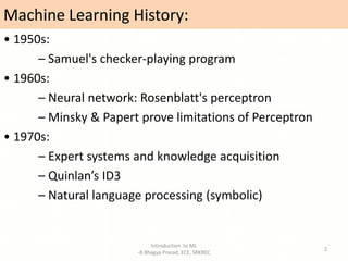
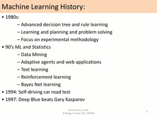
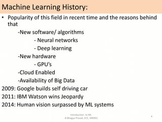
- A brief history of machine learning from the 1950s to present day.
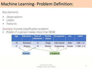
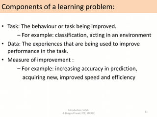
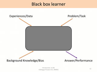
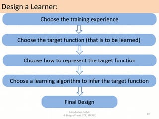
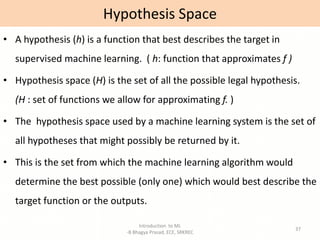
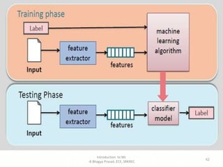
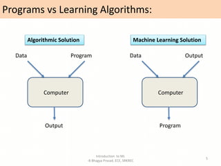
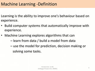
- Definitions of machine learning and the components of a learning problem.
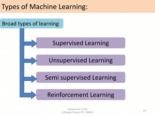
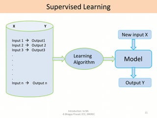
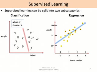
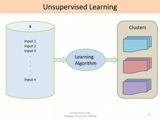
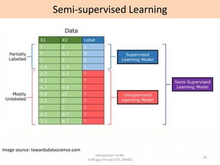
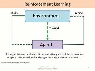
- Overviews of different types of machine learning including supervised, unsupervised, semi-supervised, and reinforcement learning.
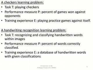
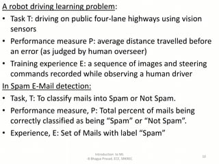
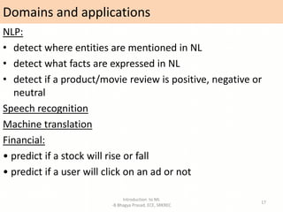
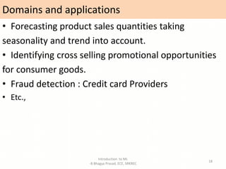
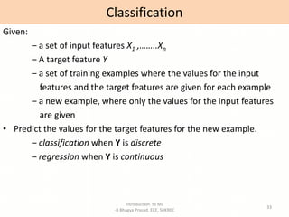
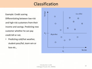
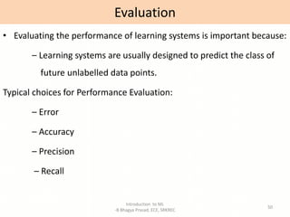
- Descriptions of common machine learning tasks like classification and regression.
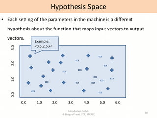
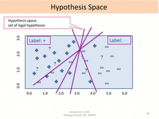
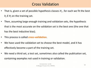
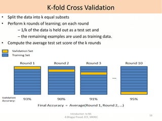
- Explanations of key machine learning concepts such as hypothesis space, inductive bias, and model performance.

![Machine Learning-Definition:
A computer program is said to learn from
experience E with respect to some class of tasks T and
performance measure P, if its performance at tasks in T, as
measured by P, improves with experience E. [Tom M.Mitchell]
Introduction to ML
-B Bhagya Prasad, ECE, SRKREC
7](https://image.slidesharecdn.com/introtoml-220417164903/85/Intro-to-ML-pptx-7-320.jpg)