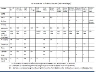
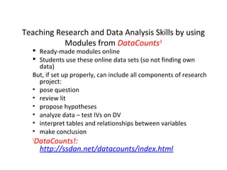
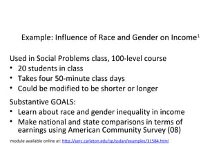
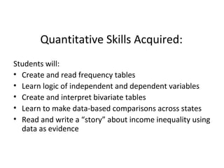
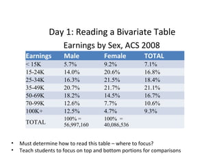
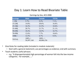
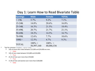
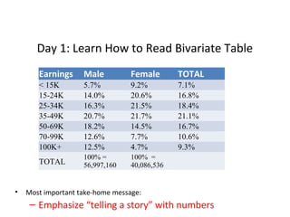
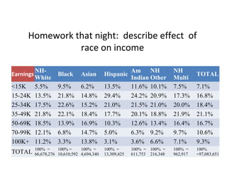
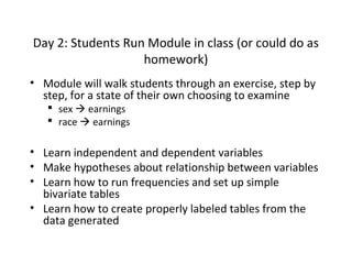
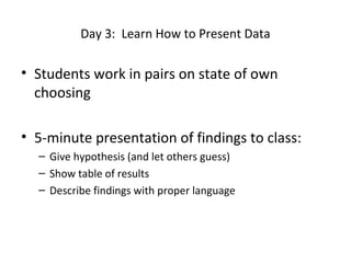
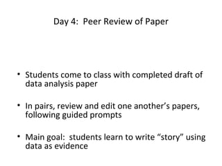
Integrating Data Analysis at Berea College
•
•

Small, liberal arts college, 3-person department
Part of NSF Integrating Data Analysis project

•

ADVANTAGES for adding data analysis:

– Small class sizes – 10-25
– students have own laptops

•

DISADVANTAGES:

– no TAs
– heavy teaching loads
•

Unusual School

– only low-income students – all full-scholarship, all
work
– often come with fairly poor prep and math skills
Quantitative Skills being taught
before and after IDA
• Until 2002, very little data analysis in courses:
–
–
–
–
–

1st year: GSS exercise in Intro
Senior year: GSS in Methods
Senior year: Collect own data in Capstone
Very little in between
Soc Majors – often math-phobes, failed pre-meds

• Saw adding QL as way to enhance research skills and
build and maintain skills across the curriculum
Integrating Data Analysis
Across our Curriculum
At beginning, our department:
• Outlined Quantitative Skills for all majors
• Mapped skills onto Courses
Teaching Research and Data Analysis Skills by using
Modules from DataCounts1

 Ready-made modules online
 Students use these online data sets (so not finding own
data)
But, if set up properly, can include all components of research
project:
• pose question
• review lit
• propose hypotheses
• analyze data – test IVs on DV
• interpret tables and relationships between variables
• make conclusion
1

DataCounts!:
http://ssdan.net/datacounts/index.html
Example: Influence of Race and Gender on Income1
Used in Social Problems class, 100-level course
• 20 students in class
• Takes four 50-minute class days
• Could be modified to be shorter or longer
Substantive GOALS:
• Learn about race and gender inequality in income
• Make national and state comparisons in terms of
earnings using American Community Survey (08)
module available online at: http://serc.carleton.edu/sp/ssdan/examples/31584.html

1
Quantitative Skills Acquired:
Students will:
• Create and read frequency tables
• Learn logic of independent and dependent variables
• Create and interpret bivariate tables
• Learn to make data-based comparisons across states
• Read and write a “story” about income inequality using
data as evidence
Day 1: How to Read Frequencies in a Handout
Reading Frequencies:
Example 1: ACS sample of full-time, year-round workers in 2008.

Male

Female

58.7 %
56,997,160

41.3 %
40,086,536

Points to make to students about a frequency table:
1. Have both percentages and numbers
2. To make comparisons, we will usually focus on the percentages
3. Percentages should add up to 100%
4. Must understand base (all full-time year-round workers in 2008)
Day 1: Start by Learning How to Read Frequencies in a
Handout
Test for common mistakes:
Sex Composition of Full-Time, Year-Round Workers, 2008
Male

Female

58.7 %
56,997,160

41.3 %
40,086,536

Which of the following is true?
A. 58.7% of the workforce is male.
B. 58.7% of men are in the workforce.
Answer: A is correct.
Day 1: Reading Frequencies

Example 2: examine earnings of full-time workers
Start by asking students to guess:
What percent of full-time workers earn over
$100,000?
<15K 15-24K 25-34K 35-49K $15,000?
What percent earn less than 50-69K 70-99K 100K+
7.1Table 2: Earnings18.4 % 21.1 % 16.7 % 10.6 2008 9.3 %
% 16.8 % for Full-Time Year-Round Workers, US, %
6,926,657 16,267,926 17,908,508 20,488,612 16,201,327 10,298,154 8,992,485
After frequencies, examine bivariate
tables
• Now ask students to guess: Who makes more,
men or women?
• How might we determine that?
• Show a bivariate table of sex and income, and
ask them to interpret:
Day 1: Reading a Bivariate Table
Earnings by Sex, ACS 2008
Earnings

Female

TOTAL

< 15K
15-24K
25-34K
35-49K
50-69K
70-99K
100K+

5.7%
14.0%
16.3%
20.7%
18.2%
12.6%
12.5%

9.2%
20.6%
21.5%
21.7%
14.5%
7.7%
4.7%

7.1%
16.8%
18.4%
21.1%
16.7%
10.6%
9.3%

TOTAL
•
•

Male

100% =
56,997,160

100% =
40,086,536

Must determine how to read this table – where to focus?
Teach students to focus on top and bottom portions for comparisons
Day 1: Learn How to Read Bivariate Table
Earnings by Sex, ACS 2008
Earnings
< 15K
15-24K
25-34K
35-49K
50-69K
70-99K
100K+
TOTAL

•
•

Male
5.7%
14.0%
16.3%
20.7%
18.2%
12.6%
12.5%
100% =
56,997,160

Female
9.2%
20.6%
21.5%
21.7%
14.5%
7.7%
4.7%
100% =
40,086,536

TOTAL
7.1%
16.8%
18.4%
21.1%
16.7%
10.6%
9.3%

Give Rules for reading table (included in module materials)
– Start with a general statement; use percentages as evidence; end with summary
Teach students useful phrases:
– e.g. “A disproportionately high percentage of women fall into the low-income
categories. For example, ….”
Day 1: Learn How to Read Bivariate Table
Earnings
< 15K
15-24K
25-34K
35-49K
50-69K
70-99K
100K+
TOTAL
•

Male
Female
5.7%
9.2%
14.0% Earnings by 20.6%
Sex, ACS 2008
16.3%
21.5%
20.7%
21.7%
18.2%
14.5%
12.6%
7.7%
12.5%
4.7%
100% =
100% =
56,997,160
40,086,536

Test for common mistakes: True or False?
 14% of those who make between $15,000 and $24,000 are men.
• False
 14% of men make between $15,000 and $24,000.
• True
 25.1% of men earn more than $70,000
• True
 17.2% of men and women earn more than $100,000
• False

TOTAL
7.1%
16.8%
18.4%
21.1%
16.7%
10.6%
9.3%
Day 1: Learn How to Read Bivariate Table
Earnings

Male

Female

< 15K
15-24K
25-34K
35-49K
50-69K
70-99K
100K+
TOTAL

•

5.7%
Earnings9.2% Sex,
by
14.0%
20.6%
16.3%
21.5%
20.7%
21.7%
18.2%
14.5%
12.6%
7.7%
12.5%
4.7%
100% =
56,997,160

TOTAL

7.1%
ACS 2008
16.8%
18.4%
21.1%
16.7%
10.6%
9.3%

100% =
40,086,536

Most important take-home message:

– Emphasize “telling a story” with numbers
Homework that night: describe effect of
race on income

<15K
15-24K
25-34K
35-49K
50-69K
70-99K
100K+

NHWhite
5.5%
13.5%
17.5%
21.8%
18.5%
12.1%
11.2%

TOTAL

100% =
100% =
100% =
66,678,276 10,610,592 4,694,340

Earnings

13.5%
29.4%
21.0%
17.7%
10.3%
5.0%
3.1%

Am NH
Indian Other
11.6% 10.1%
24.2% 20.9%
21.5% 21.0%
20.1% 18.8%
12.6% 13.4%
6.3% 9.2%
3.6% 6.6%

NH
Multi
7.5%
17.3%
20.0%
21.9%
16.4%
9.7%
7.1%

100% =
13,309,425

100% = 100% =
611,753 216,348

100% =
962,917

Black

Asian

Hispanic

9.5%
21.8%
22.6%
22.1%
13.9%
6.8%
3.3%

6.2%
14.8%
15.2%
18.4%
16.9%
14.7%
13.8%

TOTAL
7.1%
16.8%
18.4%
21.1%
16.7%
10.6%
9.3%
100%
=97,083,651
Day 2: Students Run Module in class (or could do as
homework)
• Module will walk students through an exercise, step by
step, for a state of their own choosing to examine
 sex  earnings
 race  earnings

• Learn independent and dependent variables
• Make hypotheses about relationship between variables
• Learn how to run frequencies and set up simple
bivariate tables
• Learn how to create properly labeled tables from the
data generated
Day 3: Learn How to Present Data

• Students work in pairs on state of own
choosing
• 5-minute presentation of findings to class:
– Give hypothesis (and let others guess)
– Show table of results
– Describe findings with proper language
Day 4: Peer Review of Paper

• Students come to class with completed draft of
data analysis paper
• In pairs, review and edit one another’s papers,
following guided prompts
• Main goal: students learn to write “story” using
data as evidence
Assessment
A) Used 2 forms of assessment
a) pre/post-test
b) paper, graded by rubric
B) Tried to assess both skills and confidence
levels
Comparison of Pre-test to Post-test
(past four years)
Overall score on pre-test : 55 - 60%
Overall score on post-test: 80 - 94%
Assessment of Pre and Post-test:
• Great improvement in basic skills at reading and
interpreting exactly this kind of table
• Improved confidence in working with data and
numbers
Assessment of Paper:
•
•
•
•
•

Demands higher-order skills: difficult paper
Skills vary quite a bit
Peer review helpful
Allow re-writes for students with most trouble
Students report that paper is difficult, but
worth it
Comments on Student Evals
• “I worked a lot in this class, and was always taken to
the brink of overwhelmed but not crossing over. I think
this is a sign of an excellent class. The data analysis we
did was a particular challenge. I came away from the
exercise knowing I learned something completely out
of my comfort zone.”
• “Keep on trying with the Data Analysis.... we (students)
need it... no matter how badly we do not like it at
first.”
Overview of Module
• Have been using for several years, recently updated
with 2008 American Community Survey data
• Cheerleading helps – keep telling them they’re
learning useful skills
• Fun to teach– hands-on activity; improves own
engagement in teaching these content areas
• Students generally enjoy (positive evals)
• Pre/post test shows students learn skills
• Exams and papers show modules reinforces content
[truly see race and gender inequality]
• See evidence of skills in later courses

Integrating Data Analysis at Berea College

  • 1.
    Integrating Data Analysisat Berea College • • Small, liberal arts college, 3-person department Part of NSF Integrating Data Analysis project • ADVANTAGES for adding data analysis: – Small class sizes – 10-25 – students have own laptops • DISADVANTAGES: – no TAs – heavy teaching loads • Unusual School – only low-income students – all full-scholarship, all work – often come with fairly poor prep and math skills
  • 2.
    Quantitative Skills beingtaught before and after IDA • Until 2002, very little data analysis in courses: – – – – – 1st year: GSS exercise in Intro Senior year: GSS in Methods Senior year: Collect own data in Capstone Very little in between Soc Majors – often math-phobes, failed pre-meds • Saw adding QL as way to enhance research skills and build and maintain skills across the curriculum
  • 3.
    Integrating Data Analysis Acrossour Curriculum At beginning, our department: • Outlined Quantitative Skills for all majors • Mapped skills onto Courses
  • 5.
    Teaching Research andData Analysis Skills by using Modules from DataCounts1  Ready-made modules online  Students use these online data sets (so not finding own data) But, if set up properly, can include all components of research project: • pose question • review lit • propose hypotheses • analyze data – test IVs on DV • interpret tables and relationships between variables • make conclusion 1 DataCounts!: http://ssdan.net/datacounts/index.html
  • 6.
    Example: Influence ofRace and Gender on Income1 Used in Social Problems class, 100-level course • 20 students in class • Takes four 50-minute class days • Could be modified to be shorter or longer Substantive GOALS: • Learn about race and gender inequality in income • Make national and state comparisons in terms of earnings using American Community Survey (08) module available online at: http://serc.carleton.edu/sp/ssdan/examples/31584.html 1
  • 7.
    Quantitative Skills Acquired: Studentswill: • Create and read frequency tables • Learn logic of independent and dependent variables • Create and interpret bivariate tables • Learn to make data-based comparisons across states • Read and write a “story” about income inequality using data as evidence
  • 8.
    Day 1: Howto Read Frequencies in a Handout Reading Frequencies: Example 1: ACS sample of full-time, year-round workers in 2008. Male Female 58.7 % 56,997,160 41.3 % 40,086,536 Points to make to students about a frequency table: 1. Have both percentages and numbers 2. To make comparisons, we will usually focus on the percentages 3. Percentages should add up to 100% 4. Must understand base (all full-time year-round workers in 2008)
  • 9.
    Day 1: Startby Learning How to Read Frequencies in a Handout Test for common mistakes: Sex Composition of Full-Time, Year-Round Workers, 2008 Male Female 58.7 % 56,997,160 41.3 % 40,086,536 Which of the following is true? A. 58.7% of the workforce is male. B. 58.7% of men are in the workforce. Answer: A is correct.
  • 10.
    Day 1: ReadingFrequencies Example 2: examine earnings of full-time workers Start by asking students to guess: What percent of full-time workers earn over $100,000? <15K 15-24K 25-34K 35-49K $15,000? What percent earn less than 50-69K 70-99K 100K+ 7.1Table 2: Earnings18.4 % 21.1 % 16.7 % 10.6 2008 9.3 % % 16.8 % for Full-Time Year-Round Workers, US, % 6,926,657 16,267,926 17,908,508 20,488,612 16,201,327 10,298,154 8,992,485
  • 11.
    After frequencies, examinebivariate tables • Now ask students to guess: Who makes more, men or women? • How might we determine that? • Show a bivariate table of sex and income, and ask them to interpret:
  • 12.
    Day 1: Readinga Bivariate Table Earnings by Sex, ACS 2008 Earnings Female TOTAL < 15K 15-24K 25-34K 35-49K 50-69K 70-99K 100K+ 5.7% 14.0% 16.3% 20.7% 18.2% 12.6% 12.5% 9.2% 20.6% 21.5% 21.7% 14.5% 7.7% 4.7% 7.1% 16.8% 18.4% 21.1% 16.7% 10.6% 9.3% TOTAL • • Male 100% = 56,997,160 100% = 40,086,536 Must determine how to read this table – where to focus? Teach students to focus on top and bottom portions for comparisons
  • 13.
    Day 1: LearnHow to Read Bivariate Table Earnings by Sex, ACS 2008 Earnings < 15K 15-24K 25-34K 35-49K 50-69K 70-99K 100K+ TOTAL • • Male 5.7% 14.0% 16.3% 20.7% 18.2% 12.6% 12.5% 100% = 56,997,160 Female 9.2% 20.6% 21.5% 21.7% 14.5% 7.7% 4.7% 100% = 40,086,536 TOTAL 7.1% 16.8% 18.4% 21.1% 16.7% 10.6% 9.3% Give Rules for reading table (included in module materials) – Start with a general statement; use percentages as evidence; end with summary Teach students useful phrases: – e.g. “A disproportionately high percentage of women fall into the low-income categories. For example, ….”
  • 14.
    Day 1: LearnHow to Read Bivariate Table Earnings < 15K 15-24K 25-34K 35-49K 50-69K 70-99K 100K+ TOTAL • Male Female 5.7% 9.2% 14.0% Earnings by 20.6% Sex, ACS 2008 16.3% 21.5% 20.7% 21.7% 18.2% 14.5% 12.6% 7.7% 12.5% 4.7% 100% = 100% = 56,997,160 40,086,536 Test for common mistakes: True or False?  14% of those who make between $15,000 and $24,000 are men. • False  14% of men make between $15,000 and $24,000. • True  25.1% of men earn more than $70,000 • True  17.2% of men and women earn more than $100,000 • False TOTAL 7.1% 16.8% 18.4% 21.1% 16.7% 10.6% 9.3%
  • 15.
    Day 1: LearnHow to Read Bivariate Table Earnings Male Female < 15K 15-24K 25-34K 35-49K 50-69K 70-99K 100K+ TOTAL • 5.7% Earnings9.2% Sex, by 14.0% 20.6% 16.3% 21.5% 20.7% 21.7% 18.2% 14.5% 12.6% 7.7% 12.5% 4.7% 100% = 56,997,160 TOTAL 7.1% ACS 2008 16.8% 18.4% 21.1% 16.7% 10.6% 9.3% 100% = 40,086,536 Most important take-home message: – Emphasize “telling a story” with numbers
  • 16.
    Homework that night:describe effect of race on income <15K 15-24K 25-34K 35-49K 50-69K 70-99K 100K+ NHWhite 5.5% 13.5% 17.5% 21.8% 18.5% 12.1% 11.2% TOTAL 100% = 100% = 100% = 66,678,276 10,610,592 4,694,340 Earnings 13.5% 29.4% 21.0% 17.7% 10.3% 5.0% 3.1% Am NH Indian Other 11.6% 10.1% 24.2% 20.9% 21.5% 21.0% 20.1% 18.8% 12.6% 13.4% 6.3% 9.2% 3.6% 6.6% NH Multi 7.5% 17.3% 20.0% 21.9% 16.4% 9.7% 7.1% 100% = 13,309,425 100% = 100% = 611,753 216,348 100% = 962,917 Black Asian Hispanic 9.5% 21.8% 22.6% 22.1% 13.9% 6.8% 3.3% 6.2% 14.8% 15.2% 18.4% 16.9% 14.7% 13.8% TOTAL 7.1% 16.8% 18.4% 21.1% 16.7% 10.6% 9.3% 100% =97,083,651
  • 17.
    Day 2: StudentsRun Module in class (or could do as homework) • Module will walk students through an exercise, step by step, for a state of their own choosing to examine  sex  earnings  race  earnings • Learn independent and dependent variables • Make hypotheses about relationship between variables • Learn how to run frequencies and set up simple bivariate tables • Learn how to create properly labeled tables from the data generated
  • 18.
    Day 3: LearnHow to Present Data • Students work in pairs on state of own choosing • 5-minute presentation of findings to class: – Give hypothesis (and let others guess) – Show table of results – Describe findings with proper language
  • 19.
    Day 4: PeerReview of Paper • Students come to class with completed draft of data analysis paper • In pairs, review and edit one another’s papers, following guided prompts • Main goal: students learn to write “story” using data as evidence
  • 20.
    Assessment A) Used 2forms of assessment a) pre/post-test b) paper, graded by rubric B) Tried to assess both skills and confidence levels
  • 21.
    Comparison of Pre-testto Post-test (past four years) Overall score on pre-test : 55 - 60% Overall score on post-test: 80 - 94% Assessment of Pre and Post-test: • Great improvement in basic skills at reading and interpreting exactly this kind of table • Improved confidence in working with data and numbers
  • 22.
    Assessment of Paper: • • • • • Demandshigher-order skills: difficult paper Skills vary quite a bit Peer review helpful Allow re-writes for students with most trouble Students report that paper is difficult, but worth it
  • 23.
    Comments on StudentEvals • “I worked a lot in this class, and was always taken to the brink of overwhelmed but not crossing over. I think this is a sign of an excellent class. The data analysis we did was a particular challenge. I came away from the exercise knowing I learned something completely out of my comfort zone.” • “Keep on trying with the Data Analysis.... we (students) need it... no matter how badly we do not like it at first.”
  • 24.
    Overview of Module •Have been using for several years, recently updated with 2008 American Community Survey data • Cheerleading helps – keep telling them they’re learning useful skills • Fun to teach– hands-on activity; improves own engagement in teaching these content areas • Students generally enjoy (positive evals) • Pre/post test shows students learn skills • Exams and papers show modules reinforces content [truly see race and gender inequality] • See evidence of skills in later courses

Editor's Notes

  • #5 Notes: For all of our elective courses (students must take 5), added data analysis exercises main skill, reading percentages, understanding independent and dvs, reading and creating tables