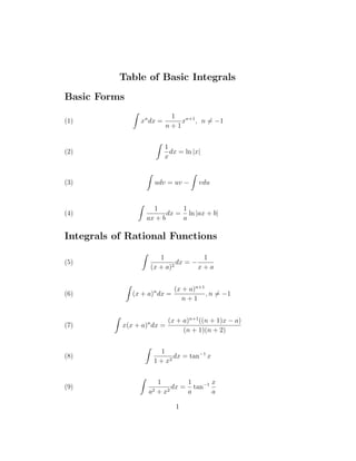
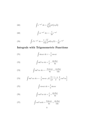
This document provides formulas for integrals of common functions including polynomials, rational functions, radicals, logarithms, exponentials, and trigonometric functions. It includes basic integral formulas like the integral of x^n dx as well as more complex integrals involving combinations of functions. There are over 100 formulas presented in a table format organized by function type.

1. Table of Basic Integrals
Basic Forms
(1) xn
dx =
1
n + 1
xn+1
, n = −1
(2)
1
x
dx = ln |x|
(3) udv = uv − vdu
(4)
1
ax + b
dx =
1
a
ln |ax + b|
Integrals of Rational Functions
(5)
1
(x + a)2
dx = −
1
x + a
(6) (x + a)n
dx =
(x + a)n+1
n + 1
, n = −1
(7) x(x + a)n
dx =
(x + a)n+1
((n + 1)x − a)
(n + 1)(n + 2)
(8)
1
1 + x2
dx = tan−1
x
(9)
1
a2 + x2
dx =
1
a
tan−1 x
a
1

2. (10)
x
a2 + x2
dx =
1
2
ln |a2
+ x2
|
(11)
x2
a2 + x2
dx = x − a tan−1 x
a
(12)
x3
a2 + x2
dx =
1
2
x2
−
1
2
a2
ln |a2
+ x2
|
(13)
1
ax2 + bx + c
dx =
2
√
4ac − b2
tan−1 2ax + b
√
4ac − b2
(14)
1
(x + a)(x + b)
dx =
1
b − a
ln
a + x
b + x
, a = b
(15)
x
(x + a)2
dx =
a
a + x
+ ln |a + x|
(16)
x
ax2 + bx + c
dx =
1
2a
ln |ax2
+bx+c|−
b
a
√
4ac − b2
tan−1 2ax + b
√
4ac − b2
Integrals with Roots
(17)
√
x − a dx =
2
3
(x − a)3/2
(18)
1
√
x ± a
dx = 2
√
x ± a
(19)
1
√
a − x
dx = −2
√
a − x
2

3. (20) x
√
x − a dx =



2a
3
(x − a)3/2
+ 2
5
(x − a)5/2
, or
2
3
x(x − a)3/2
− 4
15
(x − a)5/2
, or
2
15
(2a + 3x)(x − a)3/2
(21)
√
ax + b dx =
2b
3a
+
2x
3
√
ax + b
(22) (ax + b)3/2
dx =
2
5a
(ax + b)5/2
(23)
x
√
x ± a
dx =
2
3
(x 2a)
√
x ± a
(24)
x
a − x
dx = − x(a − x) − a tan−1 x(a − x)
x − a
(25)
x
a + x
dx = x(a + x) − a ln
√
x +
√
x + a
(26) x
√
ax + b dx =
2
15a2
(−2b2
+ abx + 3a2
x2
)
√
ax + b
(27)
x(ax + b) dx =
1
4a3/2
(2ax + b) ax(ax + b) − b2
ln a
√
x + a(ax + b)
(28)
x3(ax + b) dx =
b
12a
−
b2
8a2x
+
x
3
x3(ax + b)+
b3
8a5/2
ln a
√
x + a(ax + b)
(29)
√
x2 ± a2 dx =
1
2
x
√
x2 ± a2 ±
1
2
a2
ln x +
√
x2 ± a2
3

4. (30)
√
a2 − x2 dx =
1
2
x
√
a2 − x2 +
1
2
a2
tan−1 x
√
a2 − x2
(31) x
√
x2 ± a2 dx =
1
3
x2
± a2 3/2
(32)
1
√
x2 ± a2
dx = ln x +
√
x2 ± a2
(33)
1
√
a2 − x2
dx = sin−1 x
a
(34)
x
√
x2 ± a2
dx =
√
x2 ± a2
(35)
x
√
a2 − x2
dx = −
√
a2 − x2
(36)
x2
√
x2 ± a2
dx =
1
2
x
√
x2 ± a2
1
2
a2
ln x +
√
x2 ± a2
(37)
√
ax2 + bx + c dx =
b + 2ax
4a
√
ax2 + bx + c+
4ac − b2
8a3/2
ln 2ax + b + 2 a(ax2 + bx+c)
x
√
ax2 + bx + c dx =
1
48a5/2
2
√
a
√
ax2 + bx + c −3b2
+ 2abx + 8a(c + ax2
)
+3(b3
− 4abc) ln b + 2ax + 2
√
a
√
ax2 + bx + c
(38)
4

5. (39)
1
√
ax2 + bx + c
dx =
1
√
a
ln 2ax + b + 2 a(ax2 + bx + c)
(40)
x
√
ax2 + bx + c
dx =
1
a
√
ax2 + bx + c−
b
2a3/2
ln 2ax + b + 2 a(ax2 + bx + c)
(41)
dx
(a2 + x2)3/2
=
x
a2
√
a2 + x2
Integrals with Logarithms
(42) ln ax dx = x ln ax − x
(43) x ln x dx =
1
2
x2
ln x −
x2
4
(44) x2
ln x dx =
1
3
x3
ln x −
x3
9
(45) xn
ln x dx = xn+1 ln x
n + 1
−
1
(n + 1)2
, n = −1
(46)
ln ax
x
dx =
1
2
(ln ax)2
(47)
ln x
x2
dx = −
1
x
−
ln x
x
5

6. (48) ln(ax + b) dx = x +
b
a
ln(ax + b) − x, a = 0
(49) ln(x2
+ a2
) dx = x ln(x2
+ a2
) + 2a tan−1 x
a
− 2x
(50) ln(x2
− a2
) dx = x ln(x2
− a2
) + a ln
x + a
x − a
− 2x
(51)
ln ax2
+ bx + c dx =
1
a
√
4ac − b2 tan−1 2ax + b
√
4ac − b2
−2x+
b
2a
+ x ln ax2
+ bx + c
(52) x ln(ax + b) dx =
bx
2a
−
1
4
x2
+
1
2
x2
−
b2
a2
ln(ax + b)
(53) x ln a2
− b2
x2
dx = −
1
2
x2
+
1
2
x2
−
a2
b2
ln a2
− b2
x2
(54) (ln x)2
dx = 2x − 2x ln x + x(ln x)2
(55) (ln x)3
dx = −6x + x(ln x)3
− 3x(ln x)2
+ 6x ln x
(56) x(ln x)2
dx =
x2
4
+
1
2
x2
(ln x)2
−
1
2
x2
ln x
(57) x2
(ln x)2
dx =
2x3
27
+
1
3
x3
(ln x)2
−
2
9
x3
ln x
6

7. Integrals with Exponentials
(58) eax
dx =
1
a
eax
(59)
√
xeax
dx =
1
a
√
xeax
+
i
√
π
2a3/2
erf i
√
ax , where erf(x) =
2
√
π
x
0
e−t2
dt
(60) xex
dx = (x − 1)ex
(61) xeax
dx =
x
a
−
1
a2
eax
(62) x2
ex
dx = x2
− 2x + 2 ex
(63) x2
eax
dx =
x2
a
−
2x
a2
+
2
a3
eax
(64) x3
ex
dx = x3
− 3x2
+ 6x − 6 ex
(65) xn
eax
dx =
xn
eax
a
−
n
a
xn−1
eax
dx
(66) xn
eax
dx =
(−1)n
an+1
Γ[1 + n, −ax], where Γ(a, x) =
∞
x
ta−1
e−t
dt
(67) eax2
dx = −
i
√
π
2
√
a
erf ix
√
a
7

8. (68) e−ax2
dx =
√
π
2
√
a
erf x
√
a
(69) xe−ax2
dx = −
1
2a
e−ax2
(70) x2
e−ax2
dx =
1
4
π
a3
erf(x
√
a) −
x
2a
e−ax2
Integrals with Trigonometric Functions
(71) sin ax dx = −
1
a
cos ax
(72) sin2
ax dx =
x
2
−
sin 2ax
4a
(73) sin3
ax dx = −
3 cos ax
4a
+
cos 3ax
12a
(74) sinn
ax dx = −
1
a
cos ax 2F1
1
2
,
1 − n
2
,
3
2
, cos2
ax
(75) cos ax dx =
1
a
sin ax
(76) cos2
ax dx =
x
2
+
sin 2ax
4a
(77) cos3
axdx =
3 sin ax
4a
+
sin 3ax
12a
8

9. (78) cosp
axdx = −
1
a(1 + p)
cos1+p
ax × 2F1
1 + p
2
,
1
2
,
3 + p
2
, cos2
ax
(79) cos x sin x dx =
1
2
sin2
x + c1 = −
1
2
cos2
x + c2 = −
1
4
cos 2x + c3
(80) cos ax sin bx dx =
cos[(a − b)x]
2(a − b)
−
cos[(a + b)x]
2(a + b)
, a = b
(81) sin2
ax cos bx dx = −
sin[(2a − b)x]
4(2a − b)
+
sin bx
2b
−
sin[(2a + b)x]
4(2a + b)
(82) sin2
x cos x dx =
1
3
sin3
x
(83) cos2
ax sin bx dx =
cos[(2a − b)x]
4(2a − b)
−
cos bx
2b
−
cos[(2a + b)x]
4(2a + b)
(84) cos2
ax sin ax dx = −
1
3a
cos3
ax
(85)
sin2
ax cos2
bxdx =
x
4
−
sin 2ax
8a
−
sin[2(a − b)x]
16(a − b)
+
sin 2bx
8b
−
sin[2(a + b)x]
16(a + b)
(86) sin2
ax cos2
ax dx =
x
8
−
sin 4ax
32a
(87) tan ax dx = −
1
a
ln cos ax
9

10. (88) tan2
ax dx = −x +
1
a
tan ax
(89) tann
ax dx =
tann+1
ax
a(1 + n)
× 2F1
n + 1
2
, 1,
n + 3
2
, − tan2
ax
(90) tan3
axdx =
1
a
ln cos ax +
1
2a
sec2
ax
(91) sec x dx = ln | sec x + tan x| = 2 tanh−1
tan
x
2
(92) sec2
ax dx =
1
a
tan ax
(93) sec3
x dx =
1
2
sec x tan x +
1
2
ln | sec x + tan x|
(94) sec x tan x dx = sec x
(95) sec2
x tan x dx =
1
2
sec2
x
(96) secn
x tan x dx =
1
n
secn
x, n = 0
(97) csc x dx = ln tan
x
2
= ln | csc x − cot x| + C
10

11. (98) csc2
ax dx = −
1
a
cot ax
(99) csc3
x dx = −
1
2
cot x csc x +
1
2
ln | csc x − cot x|
(100) cscn
x cot x dx = −
1
n
cscn
x, n = 0
(101) sec x csc x dx = ln | tan x|
Products of Trigonometric Functions and Mono-
mials
(102) x cos x dx = cos x + x sin x
(103) x cos ax dx =
1
a2
cos ax +
x
a
sin ax
(104) x2
cos x dx = 2x cos x + x2
− 2 sin x
(105) x2
cos ax dx =
2x cos ax
a2
+
a2
x2
− 2
a3
sin ax
(106) xn
cos xdx = −
1
2
(i)n+1
[Γ(n + 1, −ix) + (−1)n
Γ(n + 1, ix)]
11

12. (107) xn
cos ax dx =
1
2
(ia)1−n
[(−1)n
Γ(n + 1, −iax) − Γ(n + 1, ixa)]
(108) x sin x dx = −x cos x + sin x
(109) x sin ax dx = −
x cos ax
a
+
sin ax
a2
(110) x2
sin x dx = 2 − x2
cos x + 2x sin x
(111) x2
sin ax dx =
2 − a2
x2
a3
cos ax +
2x sin ax
a2
(112) xn
sin x dx = −
1
2
(i)n
[Γ(n + 1, −ix) − (−1)n
Γ(n + 1, −ix)]
(113) x cos2
x dx =
x2
4
+
1
8
cos 2x +
1
4
x sin 2x
(114) x sin2
x dx =
x2
4
−
1
8
cos 2x −
1
4
x sin 2x
(115) x tan2
x dx = −
x2
2
+ ln cos x + x tan x
(116) x sec2
x dx = ln cos x + x tan x
12

13. Products of Trigonometric Functions and Ex-
ponentials
(117) ex
sin x dx =
1
2
ex
(sin x − cos x)
(118) ebx
sin ax dx =
1
a2 + b2
ebx
(b sin ax − a cos ax)
(119) ex
cos x dx =
1
2
ex
(sin x + cos x)
(120) ebx
cos ax dx =
1
a2 + b2
ebx
(a sin ax + b cos ax)
(121) xex
sin x dx =
1
2
ex
(cos x − x cos x + x sin x)
(122) xex
cos x dx =
1
2
ex
(x cos x − sin x + x sin x)
Integrals of Hyperbolic Functions
(123) cosh ax dx =
1
a
sinh ax
(124) eax
cosh bx dx =



eax
a2 − b2
[a cosh bx − b sinh bx] a = b
e2ax
4a
+
x
2
a = b
(125) sinh ax dx =
1
a
cosh ax
13

14. (126) eax
sinh bx dx =



eax
a2 − b2
[−b cosh bx + a sinh bx] a = b
e2ax
4a
−
x
2
a = b
(127) tanh axdx =
1
a
ln cosh ax
(128) eax
tanh bx dx =



e(a+2b)x
(a + 2b)
2F1 1 +
a
2b
, 1, 2 +
a
2b
, −e2bx
−
1
a
eax
2F1 1,
a
2b
, 1 +
a
2b
, −e2bx
a = b
eax
− 2 tan−1
[eax
]
a
a = b
(129) cos ax cosh bx dx =
1
a2 + b2
[a sin ax cosh bx + b cos ax sinh bx]
(130) cos ax sinh bx dx =
1
a2 + b2
[b cos ax cosh bx + a sin ax sinh bx]
(131) sin ax cosh bx dx =
1
a2 + b2
[−a cos ax cosh bx + b sin ax sinh bx]
(132) sin ax sinh bx dx =
1
a2 + b2
[b cosh bx sin ax − a cos ax sinh bx]
(133) sinh ax cosh axdx =
1
4a
[−2ax + sinh 2ax]
(134) sinh ax cosh bx dx =
1
b2 − a2
[b cosh bx sinh ax − a cosh ax sinh bx]
c 2014. From http://integral-table.com, last revised June 14, 2014. This mate-
rial is provided as is without warranty or representation about the accuracy, correctness or
suitability of this material for any purpose. This work is licensed under the Creative Com-
mons Attribution-Noncommercial-Share Alike 3.0 United States License. To view a copy
of this license, visit http://creativecommons.org/licenses/by-nc-sa/3.0/ or send
a letter to Creative Commons, 171 Second Street, Suite 300, San Francisco, California,
94105, USA.
14