Download as PDF, PPTX
![> me
$name
[1] "Takashi Kitano"
$twitter
[1] "@kashitan"
$work_in
[1] " "](https://image.slidesharecdn.com/20180421tokyor69full-190628110634/75/tidygraph-ggraph-ver-2-2048.jpg)


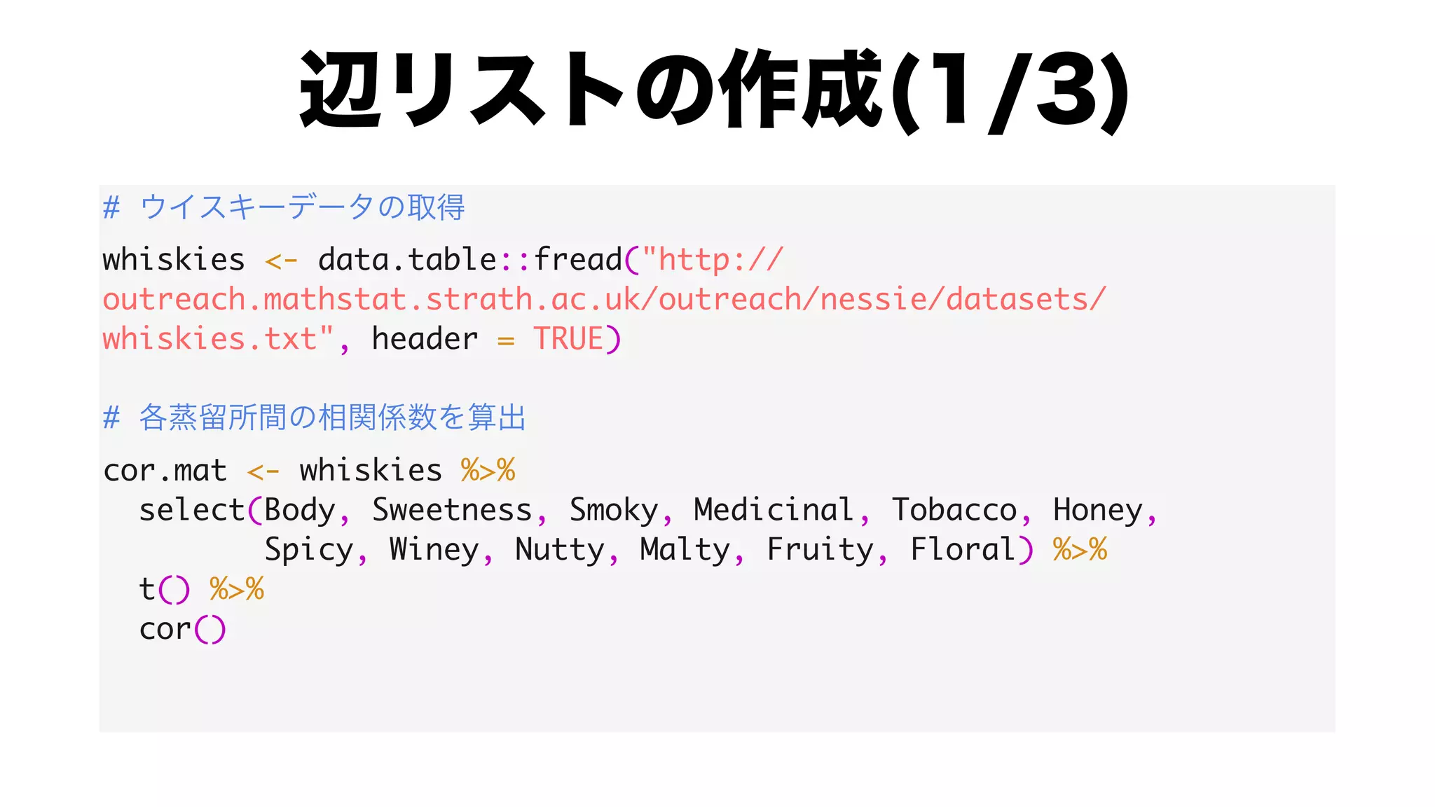
![#
colnames(cor.mat) <- whiskies$Distillery
rownames(cor.mat) <- whiskies$Distillery
#
cor.mat[upper.tri(cor.mat, diag = TRUE)] <- NA
cor.mat[1:5, 1:5]
Aberfeldy Aberlour AnCnoc Ardbeg Ardmore
Aberfeldy NA NA NA NA NA
Aberlour 0.7086322 NA NA NA NA
AnCnoc 0.6973541 0.5030737 NA NA NA
Ardbeg -0.1473114 -0.2285909 -0.1404355 NA NA
Ardmore 0.7319024 0.5118338 0.5570195 0.2316174 NA](https://image.slidesharecdn.com/20180421tokyor69full-190628110634/75/tidygraph-ggraph-ver-31-2048.jpg)


![#
g %>% igraph::graph.density()
[1] 0.06105834
#
g %>% igraph::transitivity()
[1] 0.2797927
# ( 1)
g %>% igraph::reciprocity()
[1] 1](https://image.slidesharecdn.com/20180421tokyor69full-190628110634/75/tidygraph-ggraph-ver-38-2048.jpg)


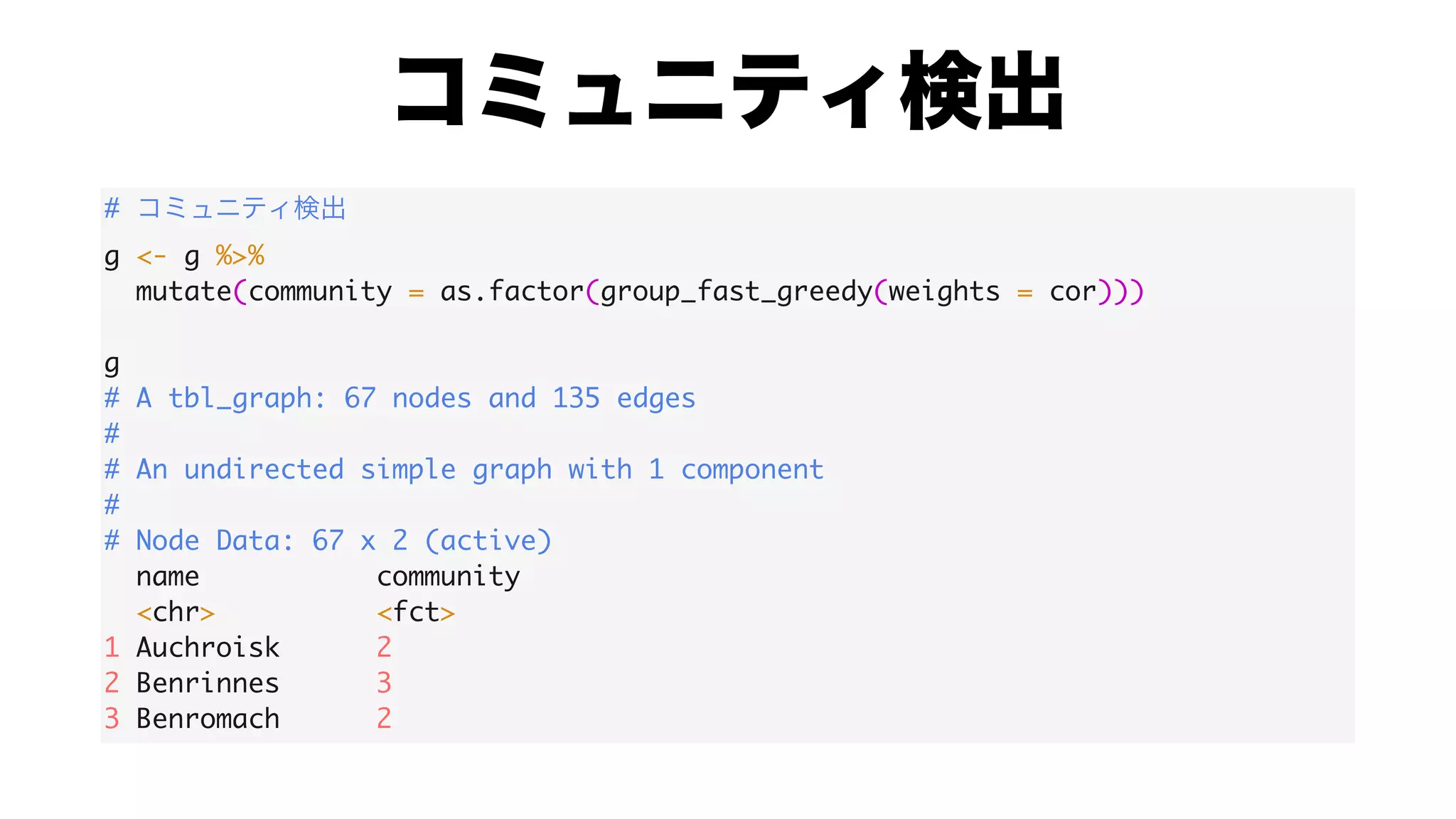


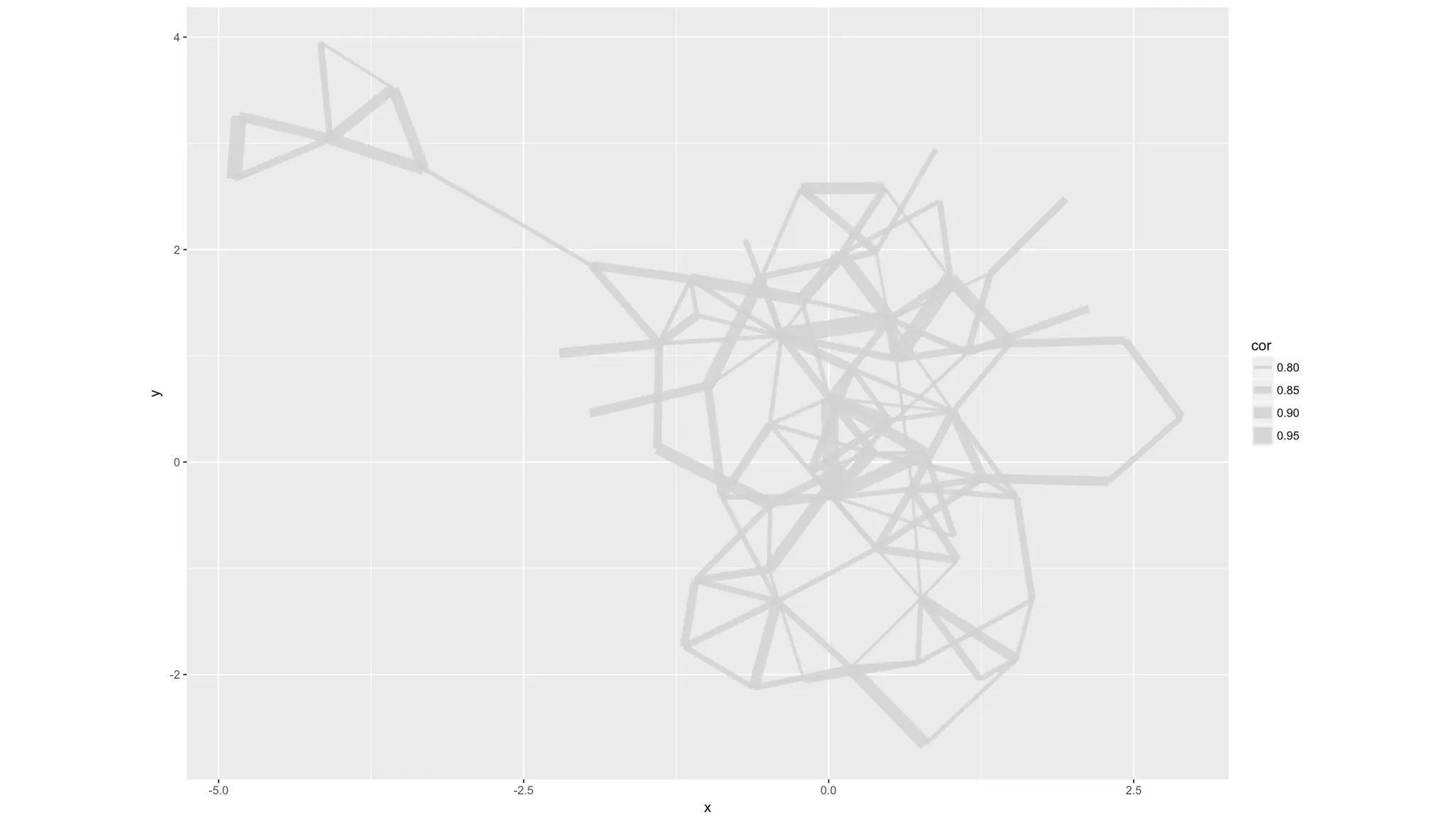


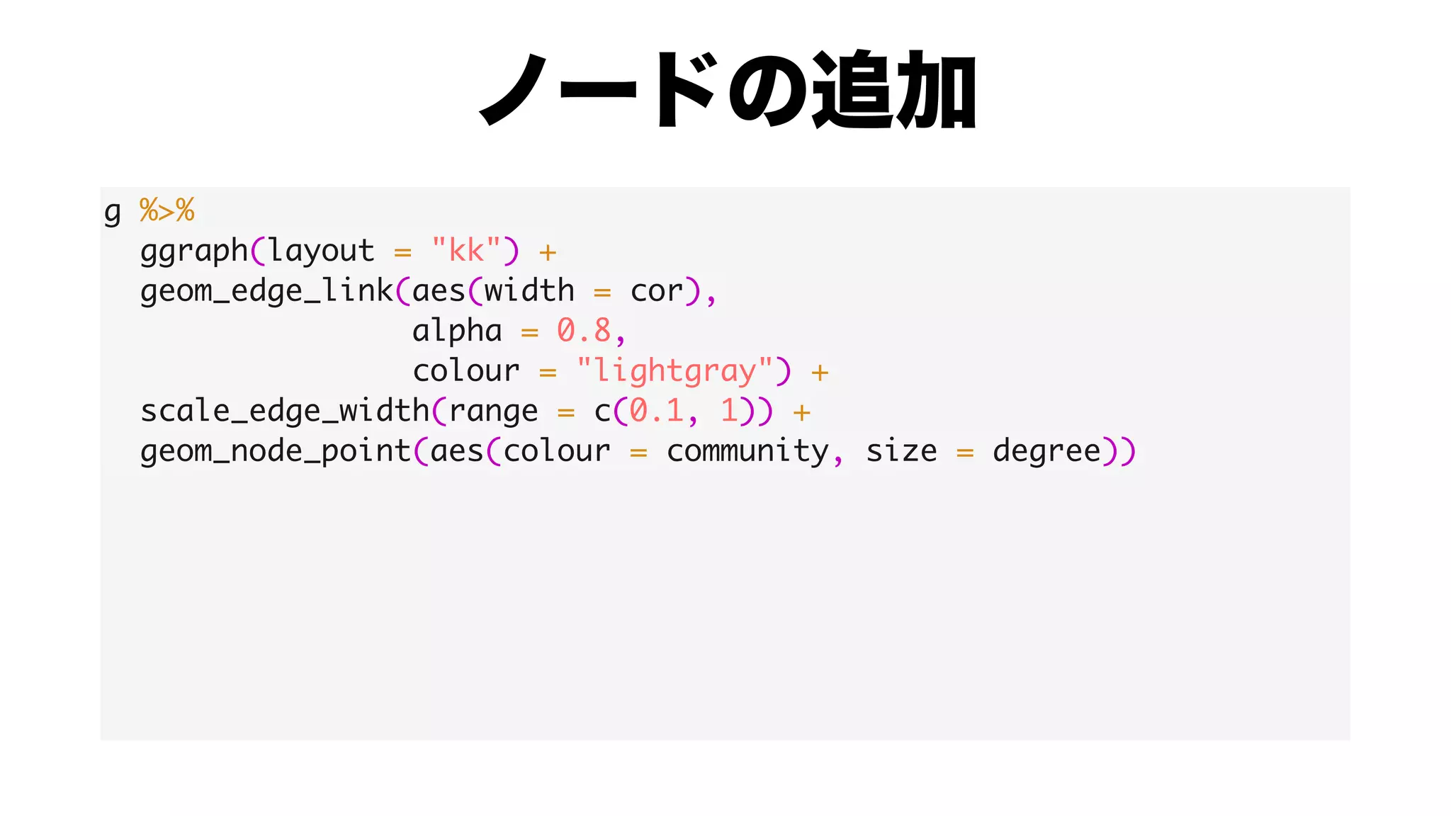


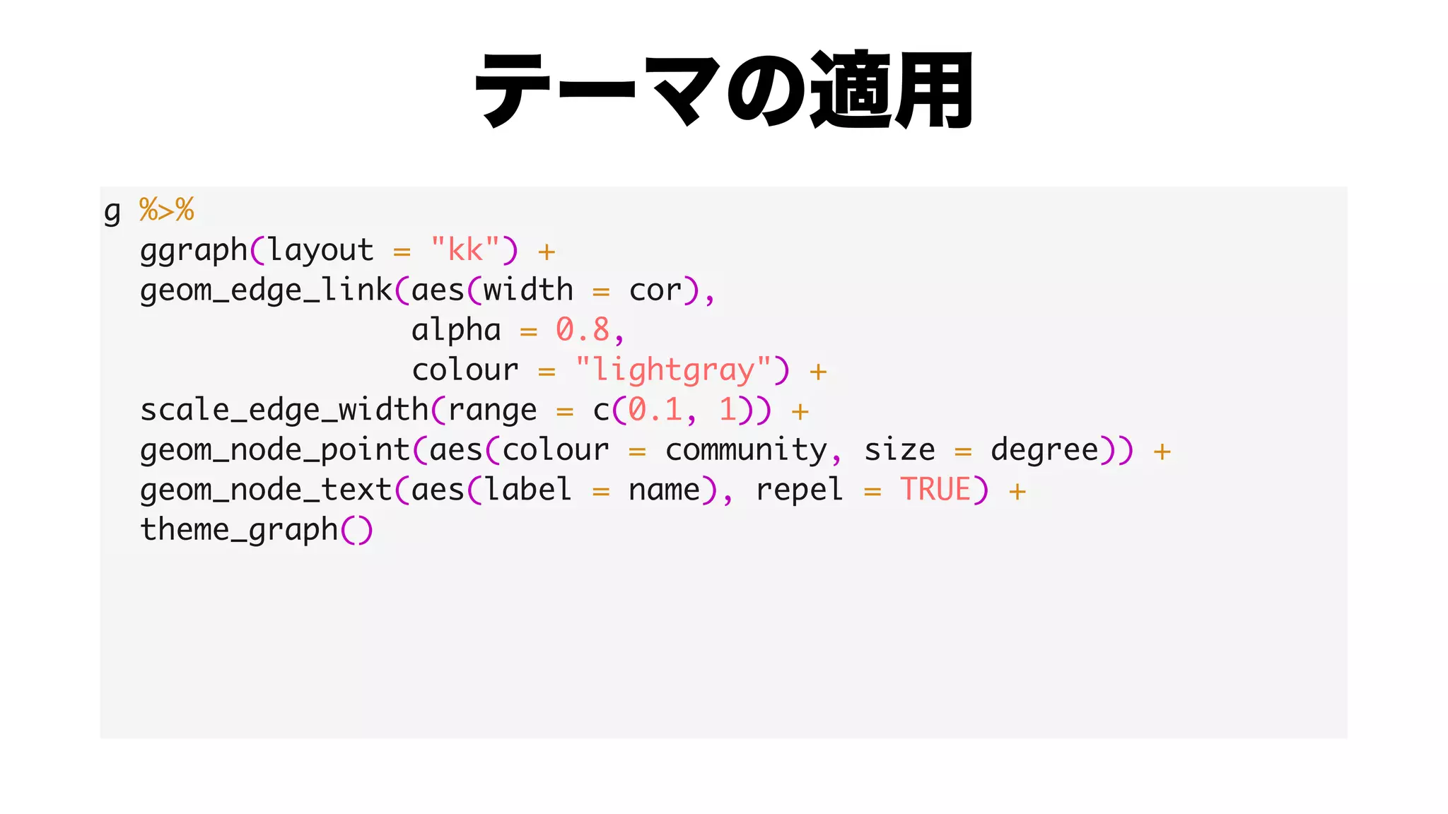
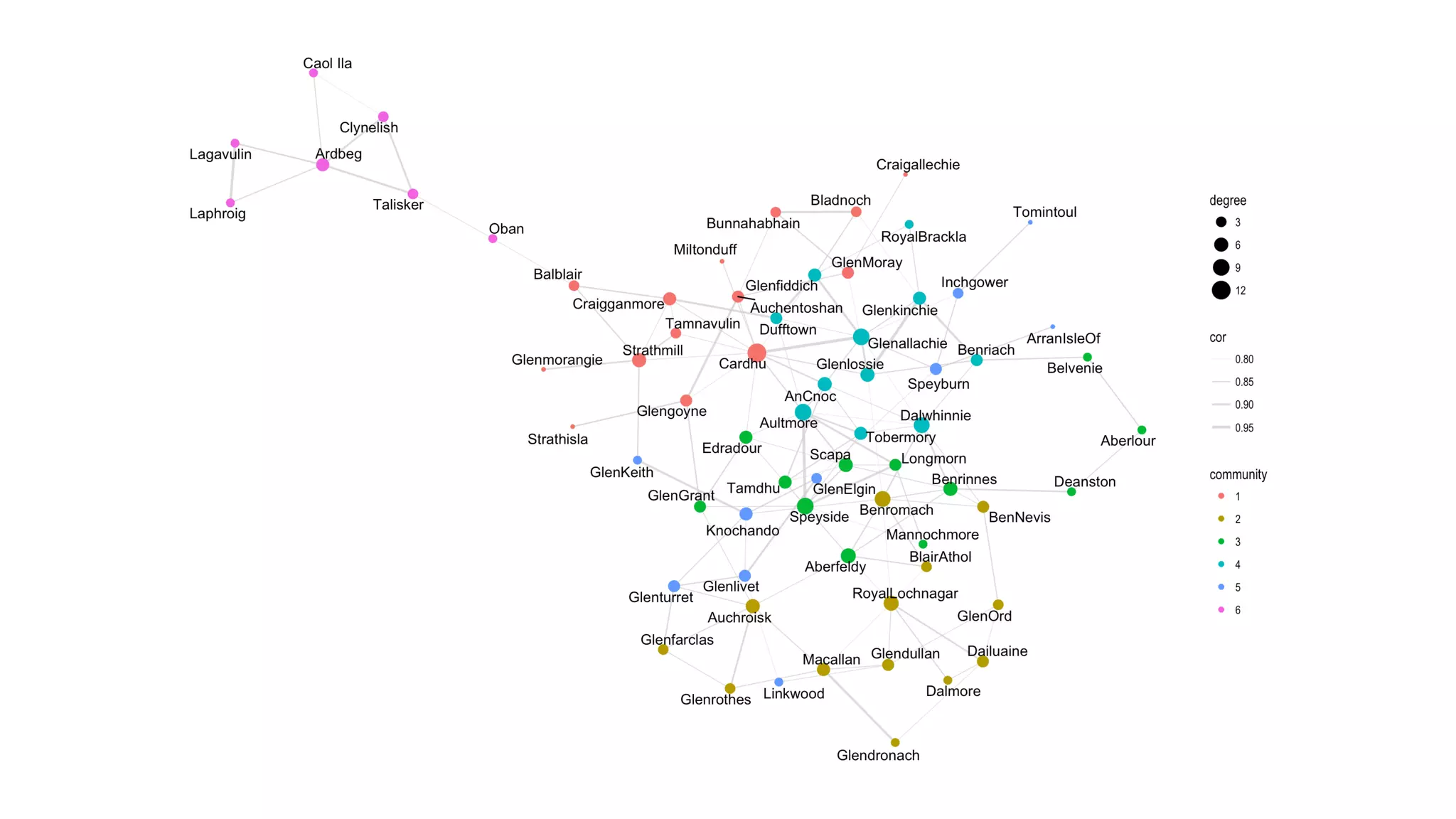


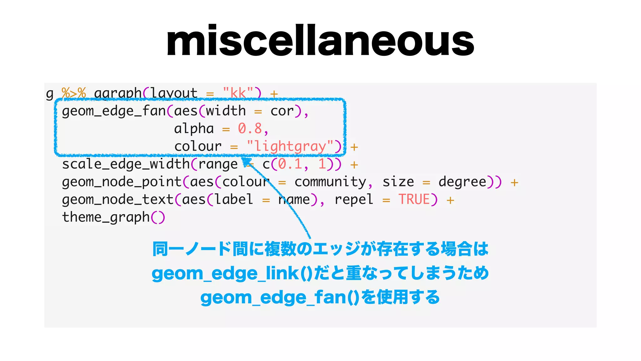


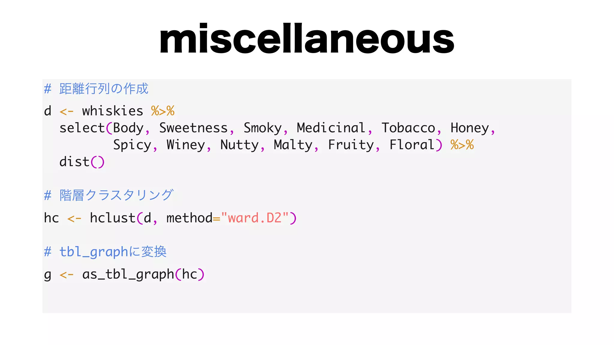


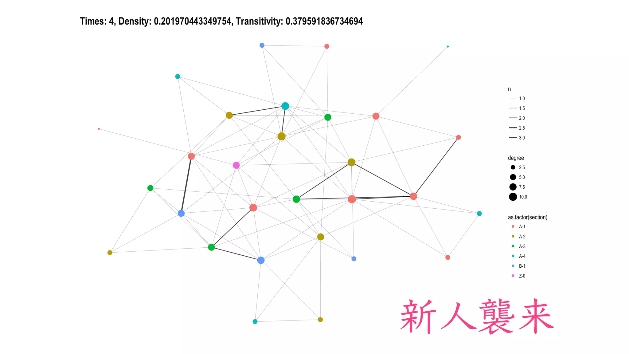
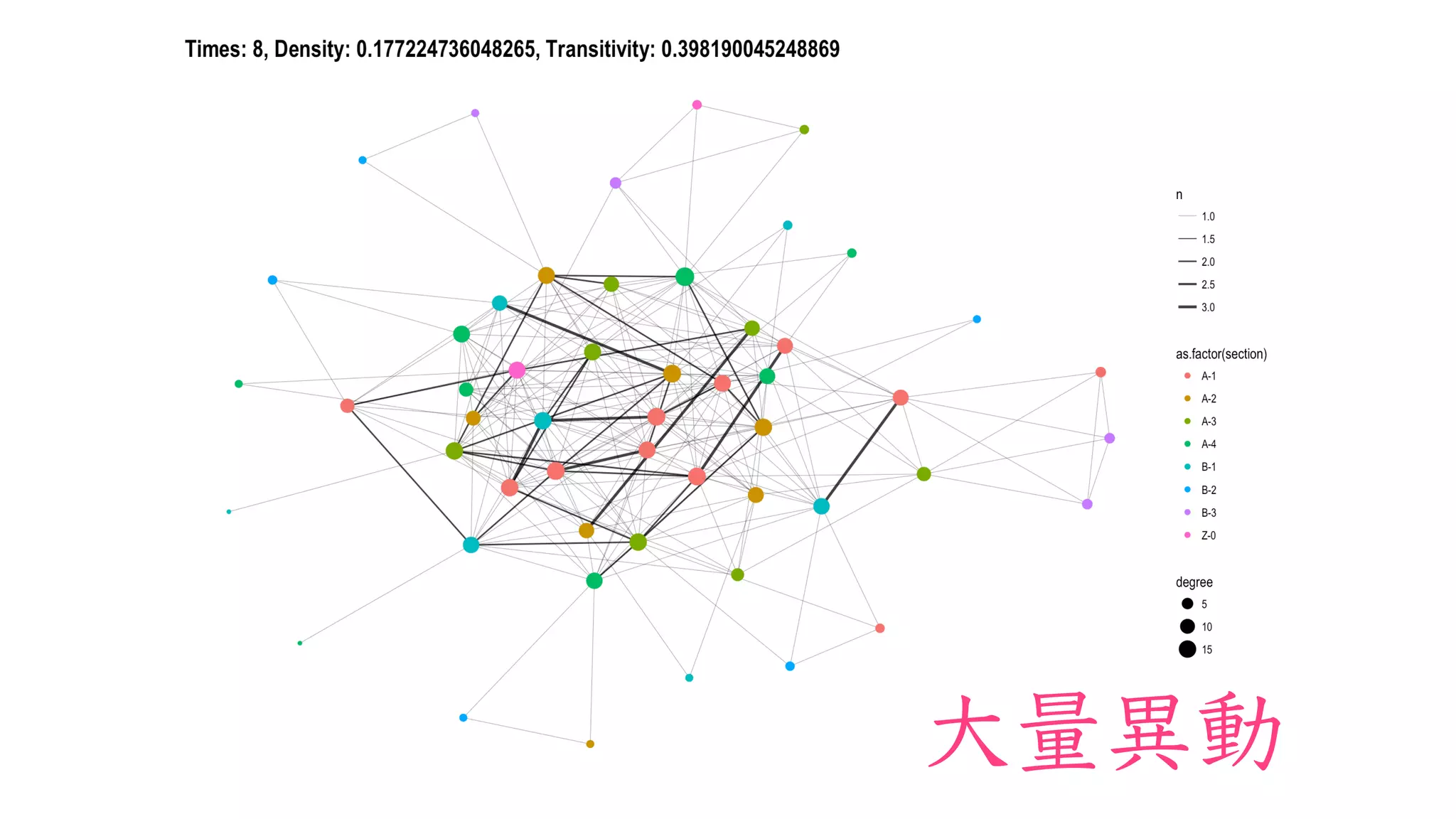


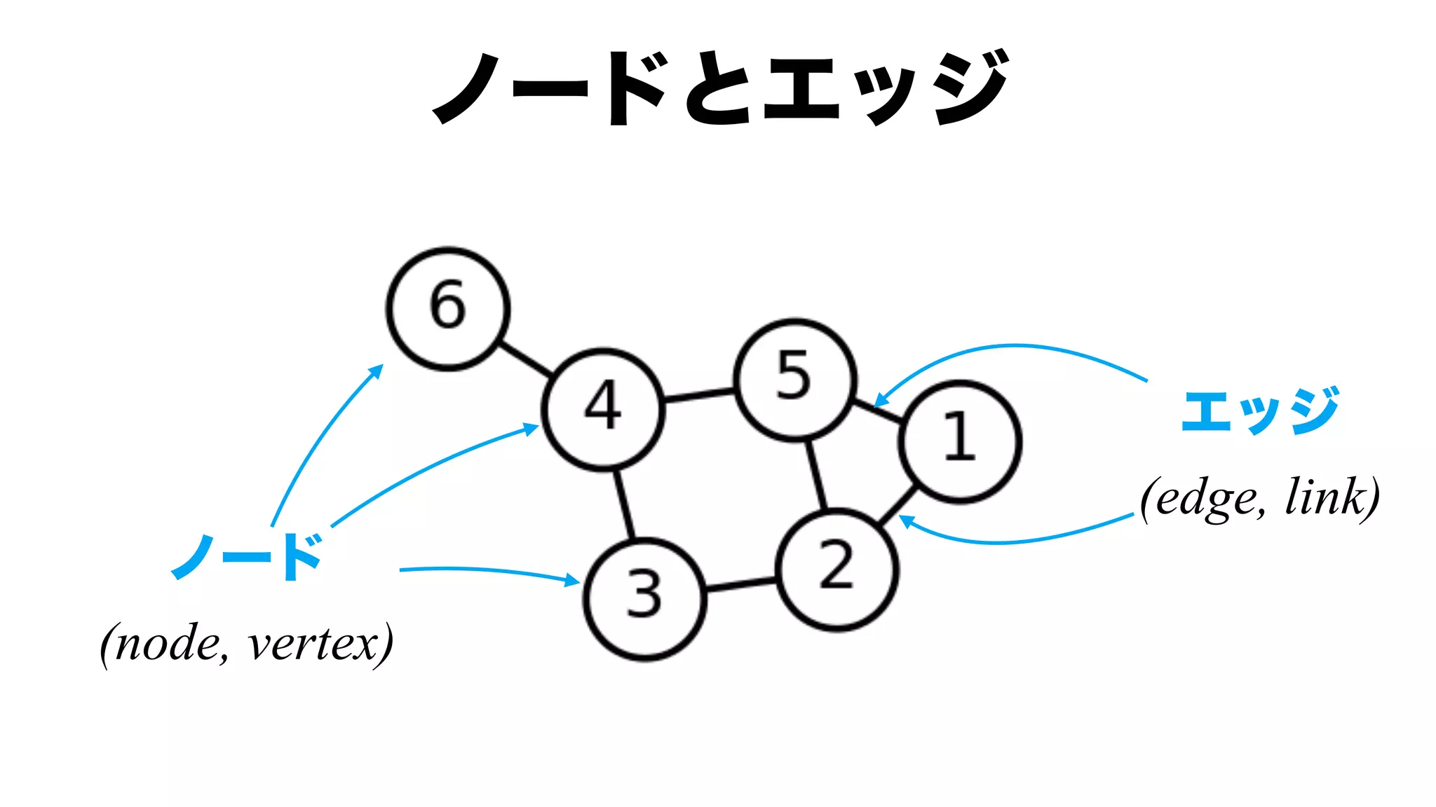
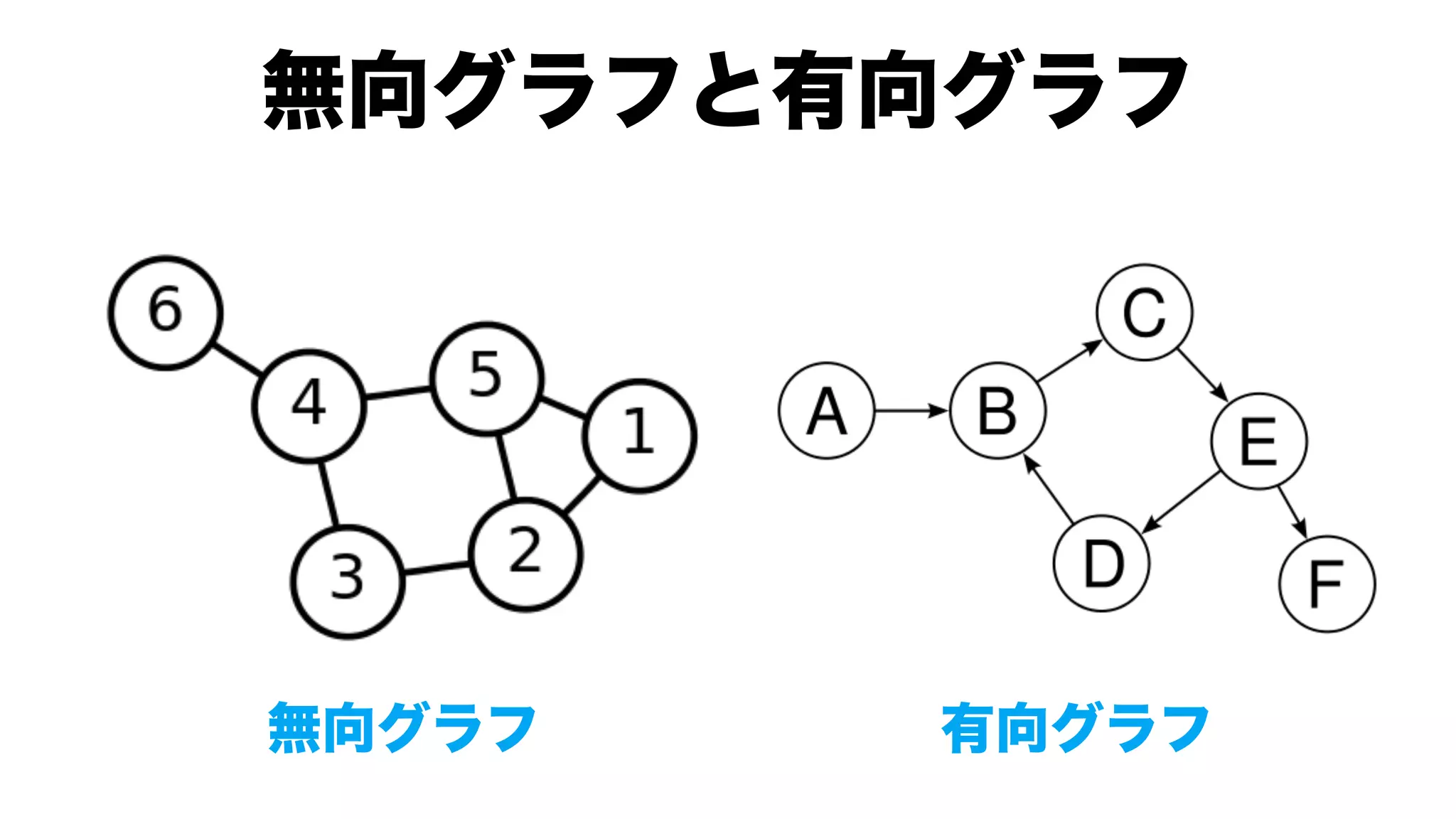
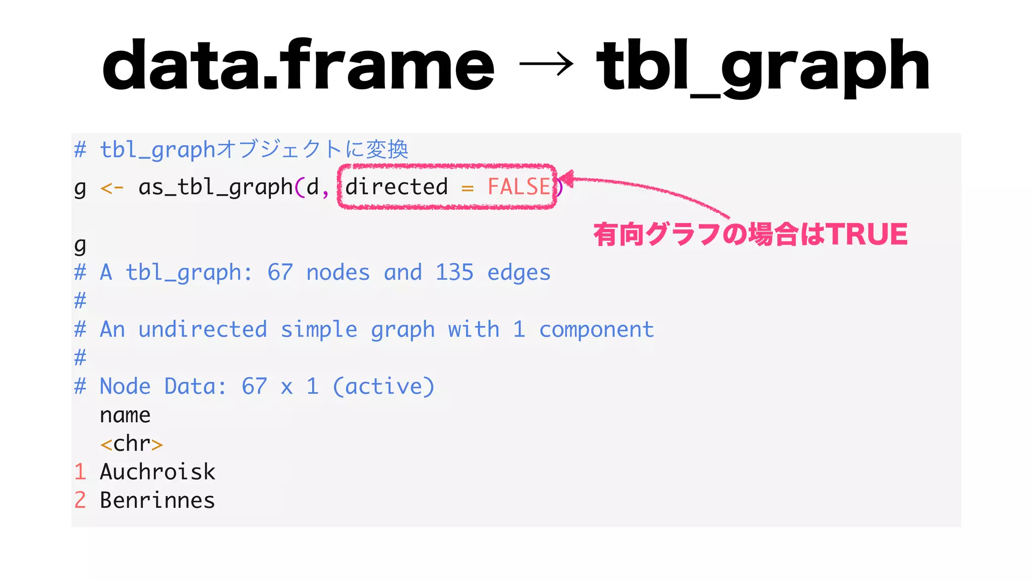
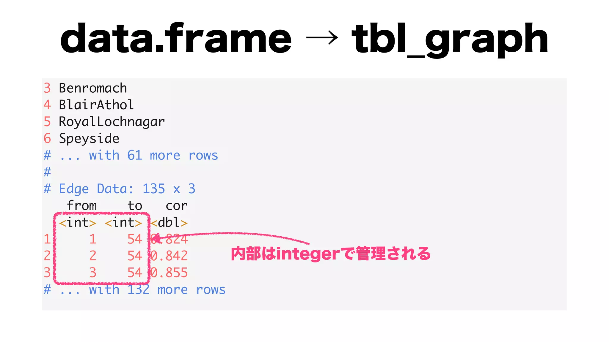
The document discusses analyzing correlation networks between Scottish whisky distilleries. A correlation matrix is created from sensory characteristics of whiskies. This is converted to a graph object where nodes are distilleries and edges represent correlations above 0.8. The graph is analyzed to find clustering of distilleries based on sensory profiles and key central nodes. Visualizations of the network are also created.


![[DSC Europe 25] Jim Sterne - Adopting Generative AI Capabilities Into the Ent...](https://cdn.slidesharecdn.com/ss_thumbnails/sxhpofuorcagxsaulkmt-3-251204082258-7e66bc48-thumbnail.jpg?width=640&height=640&fit=bounds)
![[DSC Europe 25] Nikola Rajovic - Hardware Technologies Under the Hood: RISC-V...](https://cdn.slidesharecdn.com/ss_thumbnails/o2gptrmtoyqndgoshwgq-dsc2025-tenstorrent-rajovic-251205090438-814685f5-thumbnail.jpg?width=640&height=640&fit=bounds)
![[DSC Europe 25] Max Talanov - Non digital NNs.pptx](https://cdn.slidesharecdn.com/ss_thumbnails/wif8tr3gtua74qvtopke-non-digital-nns-251205090438-26b0eea6-thumbnail.jpg?width=640&height=640&fit=bounds)


![[DSC Europe 25] Dragan Vucic - Building the Learning Organization - How AI Tr...](https://cdn.slidesharecdn.com/ss_thumbnails/8brigo2sbu6qur6gxrra-7-251205085715-6ae07d24-thumbnail.jpg?width=640&height=640&fit=bounds)

![[DSC Europe 25] Marija Vlajkovic & Andrea Radonjanin - Integration of AI tool...](https://cdn.slidesharecdn.com/ss_thumbnails/qf1jrglttoc3bm8s3aop-final-integration-of-ai-tools-251208151905-394f3a6a-thumbnail.jpg?width=640&height=640&fit=bounds)

