Downloaded 21 times


![Integrals with Exponentials
(58) eax
dx =
1
a
eax
(59)
√
xeax
dx =
1
a
√
xeax
+
i
√
π
2a3/2
erf i
√
ax , where erf(x) =
2
√
π
x
0
e−t2
dt
(60) xex
dx = (x − 1)ex
(61) xeax
dx =
x
a
−
1
a2
eax
(62) x2
ex
dx = x2
− 2x + 2 ex
(63) x2
eax
dx =
x2
a
−
2x
a2
+
2
a3
eax
(64) x3
ex
dx = x3
− 3x2
+ 6x − 6 ex
(65) xn
eax
dx =
xn
eax
a
−
n
a
xn−1
eax
dx
(66) xn
eax
dx =
(−1)n
an+1
Γ[1 + n, −ax], where Γ(a, x) =
∞
x
ta−1
e−t
dt
(67) eax2
dx = −
i
√
π
2
√
a
erf ix
√
a
7](https://image.slidesharecdn.com/integral-table-140816135445-phpapp01/85/Integral-table-7-320.jpg)

![(78) cosp
axdx = −
1
a(1 + p)
cos1+p
ax × 2F1
1 + p
2
,
1
2
,
3 + p
2
, cos2
ax
(79) cos x sin x dx =
1
2
sin2
x + c1 = −
1
2
cos2
x + c2 = −
1
4
cos 2x + c3
(80) cos ax sin bx dx =
cos[(a − b)x]
2(a − b)
−
cos[(a + b)x]
2(a + b)
, a = b
(81) sin2
ax cos bx dx = −
sin[(2a − b)x]
4(2a − b)
+
sin bx
2b
−
sin[(2a + b)x]
4(2a + b)
(82) sin2
x cos x dx =
1
3
sin3
x
(83) cos2
ax sin bx dx =
cos[(2a − b)x]
4(2a − b)
−
cos bx
2b
−
cos[(2a + b)x]
4(2a + b)
(84) cos2
ax sin ax dx = −
1
3a
cos3
ax
(85)
sin2
ax cos2
bxdx =
x
4
−
sin 2ax
8a
−
sin[2(a − b)x]
16(a − b)
+
sin 2bx
8b
−
sin[2(a + b)x]
16(a + b)
(86) sin2
ax cos2
ax dx =
x
8
−
sin 4ax
32a
(87) tan ax dx = −
1
a
ln cos ax
9](https://image.slidesharecdn.com/integral-table-140816135445-phpapp01/85/Integral-table-9-320.jpg)

![(98) csc2
ax dx = −
1
a
cot ax
(99) csc3
x dx = −
1
2
cot x csc x +
1
2
ln | csc x − cot x|
(100) cscn
x cot x dx = −
1
n
cscn
x, n = 0
(101) sec x csc x dx = ln | tan x|
Products of Trigonometric Functions and Mono-
mials
(102) x cos x dx = cos x + x sin x
(103) x cos ax dx =
1
a2
cos ax +
x
a
sin ax
(104) x2
cos x dx = 2x cos x + x2
− 2 sin x
(105) x2
cos ax dx =
2x cos ax
a2
+
a2
x2
− 2
a3
sin ax
(106) xn
cos xdx = −
1
2
(i)n+1
[Γ(n + 1, −ix) + (−1)n
Γ(n + 1, ix)]
11](https://image.slidesharecdn.com/integral-table-140816135445-phpapp01/85/Integral-table-11-320.jpg)
![(107) xn
cos ax dx =
1
2
(ia)1−n
[(−1)n
Γ(n + 1, −iax) − Γ(n + 1, ixa)]
(108) x sin x dx = −x cos x + sin x
(109) x sin ax dx = −
x cos ax
a
+
sin ax
a2
(110) x2
sin x dx = 2 − x2
cos x + 2x sin x
(111) x2
sin ax dx =
2 − a2
x2
a3
cos ax +
2x sin ax
a2
(112) xn
sin x dx = −
1
2
(i)n
[Γ(n + 1, −ix) − (−1)n
Γ(n + 1, −ix)]
(113) x cos2
x dx =
x2
4
+
1
8
cos 2x +
1
4
x sin 2x
(114) x sin2
x dx =
x2
4
−
1
8
cos 2x −
1
4
x sin 2x
(115) x tan2
x dx = −
x2
2
+ ln cos x + x tan x
(116) x sec2
x dx = ln cos x + x tan x
12](https://image.slidesharecdn.com/integral-table-140816135445-phpapp01/85/Integral-table-12-320.jpg)
![Products of Trigonometric Functions and Ex-
ponentials
(117) ex
sin x dx =
1
2
ex
(sin x − cos x)
(118) ebx
sin ax dx =
1
a2 + b2
ebx
(b sin ax − a cos ax)
(119) ex
cos x dx =
1
2
ex
(sin x + cos x)
(120) ebx
cos ax dx =
1
a2 + b2
ebx
(a sin ax + b cos ax)
(121) xex
sin x dx =
1
2
ex
(cos x − x cos x + x sin x)
(122) xex
cos x dx =
1
2
ex
(x cos x − sin x + x sin x)
Integrals of Hyperbolic Functions
(123) cosh ax dx =
1
a
sinh ax
(124) eax
cosh bx dx =
eax
a2 − b2
[a cosh bx − b sinh bx] a = b
e2ax
4a
+
x
2
a = b
(125) sinh ax dx =
1
a
cosh ax
13](https://image.slidesharecdn.com/integral-table-140816135445-phpapp01/85/Integral-table-13-320.jpg)
![(126) eax
sinh bx dx =
eax
a2 − b2
[−b cosh bx + a sinh bx] a = b
e2ax
4a
−
x
2
a = b
(127) tanh axdx =
1
a
ln cosh ax
(128) eax
tanh bx dx =
e(a+2b)x
(a + 2b)
2F1 1 +
a
2b
, 1, 2 +
a
2b
, −e2bx
−
1
a
eax
2F1 1,
a
2b
, 1 +
a
2b
, −e2bx
a = b
eax
− 2 tan−1
[eax
]
a
a = b
(129) cos ax cosh bx dx =
1
a2 + b2
[a sin ax cosh bx + b cos ax sinh bx]
(130) cos ax sinh bx dx =
1
a2 + b2
[b cos ax cosh bx + a sin ax sinh bx]
(131) sin ax cosh bx dx =
1
a2 + b2
[−a cos ax cosh bx + b sin ax sinh bx]
(132) sin ax sinh bx dx =
1
a2 + b2
[b cosh bx sin ax − a cos ax sinh bx]
(133) sinh ax cosh axdx =
1
4a
[−2ax + sinh 2ax]
(134) sinh ax cosh bx dx =
1
b2 − a2
[b cosh bx sinh ax − a cosh ax sinh bx]
c 2014. From http://integral-table.com, last revised June 14, 2014. This mate-
rial is provided as is without warranty or representation about the accuracy, correctness or
suitability of this material for any purpose. This work is licensed under the Creative Com-
mons Attribution-Noncommercial-Share Alike 3.0 United States License. To view a copy
of this license, visit http://creativecommons.org/licenses/by-nc-sa/3.0/ or send
a letter to Creative Commons, 171 Second Street, Suite 300, San Francisco, California,
94105, USA.
14](https://image.slidesharecdn.com/integral-table-140816135445-phpapp01/85/Integral-table-14-320.jpg)

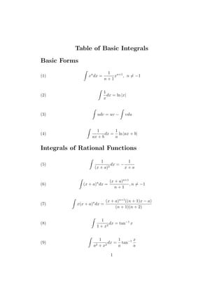
This document provides formulas for integrals of common functions including polynomials, rational functions, radicals, logarithms, exponentials, and trigonometric functions. It includes basic integral formulas like the integral of x^n dx as well as more complex integrals involving combinations of functions. There are over 100 formulas presented in a table format organized by function type.


![POLINOMIOS CICLOTÓMICOS EN CUERPOS K[X] Y RAICES PRIMITIVAS MÓDULO N](https://cdn.slidesharecdn.com/ss_thumbnails/ysque-100317201527-phpapp01-thumbnail.jpg?width=640&height=640&fit=bounds)


