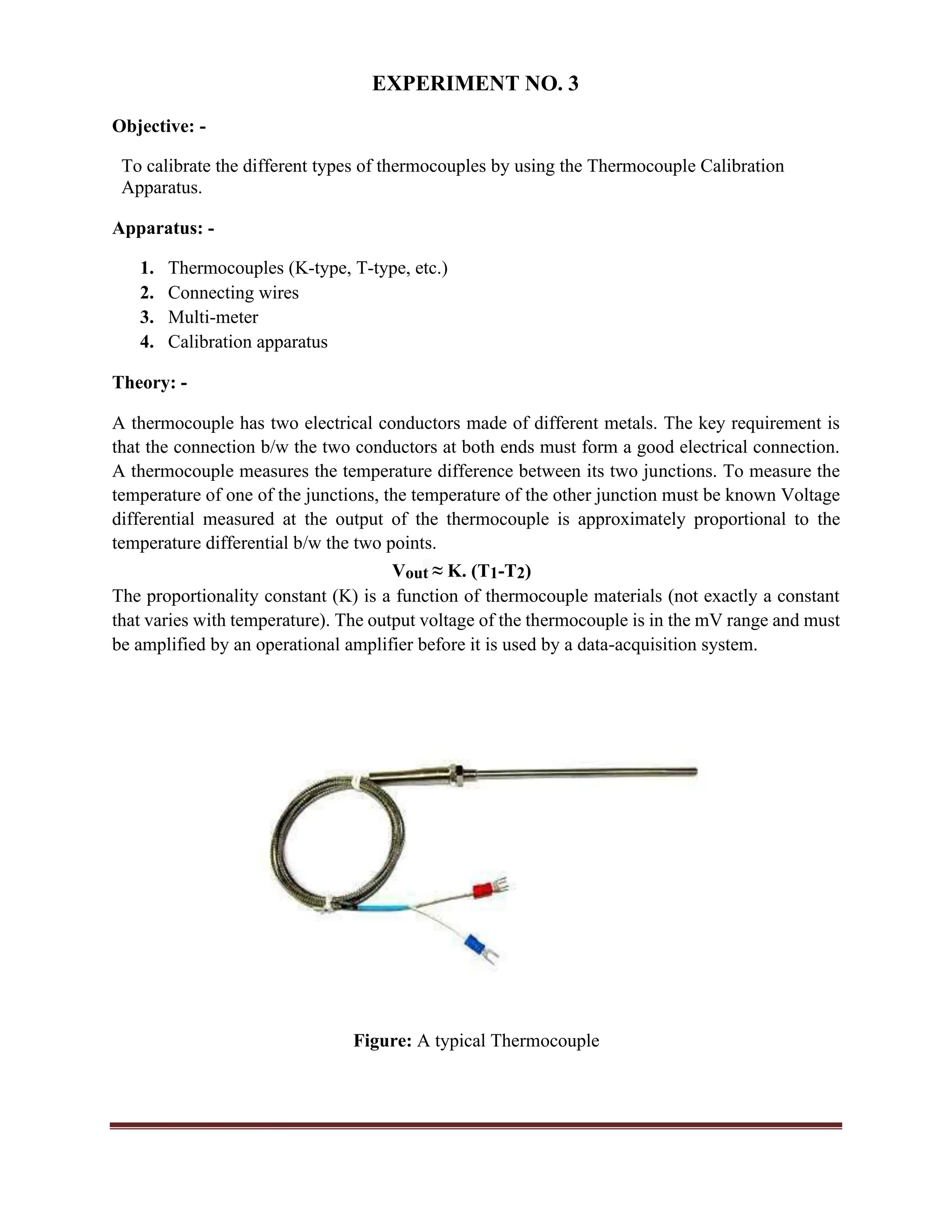
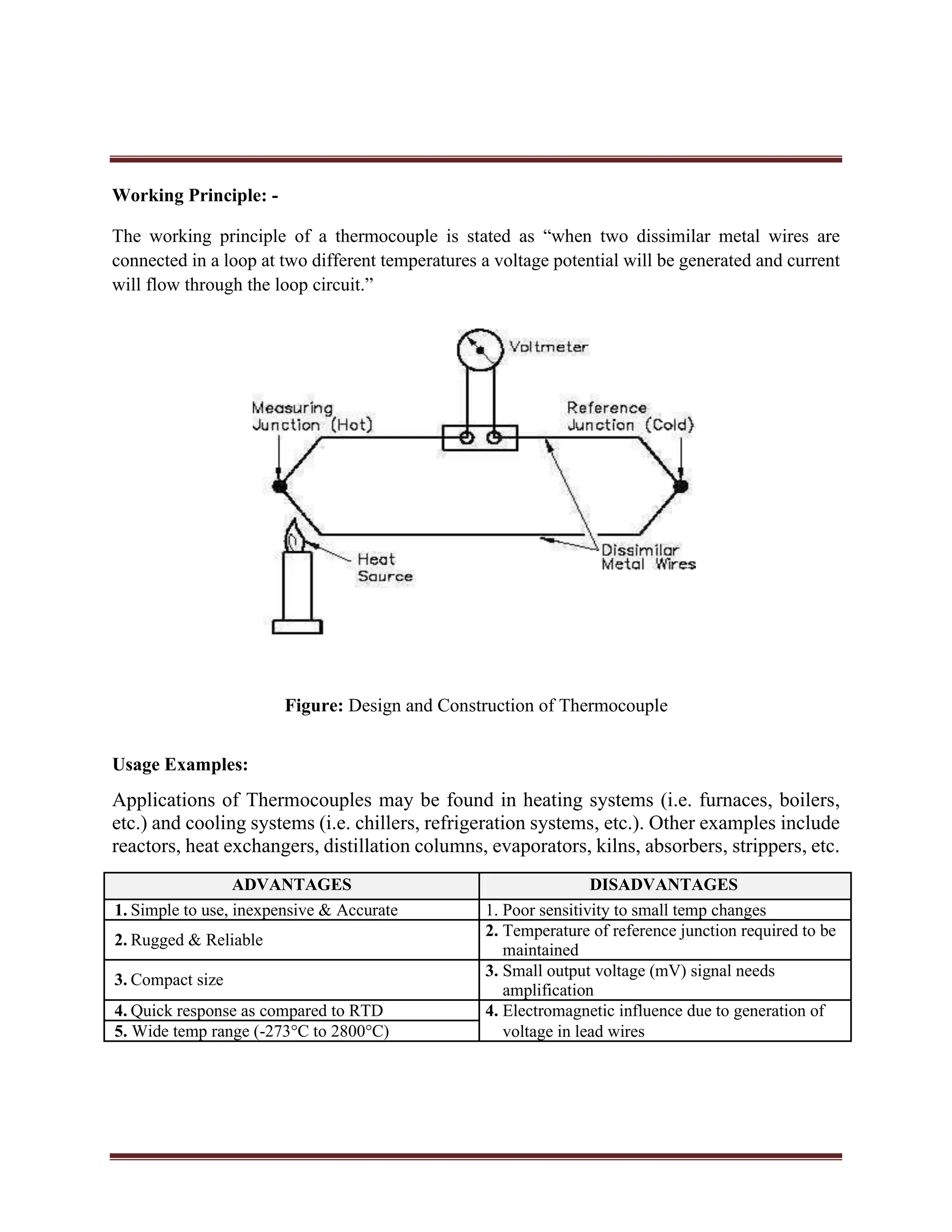
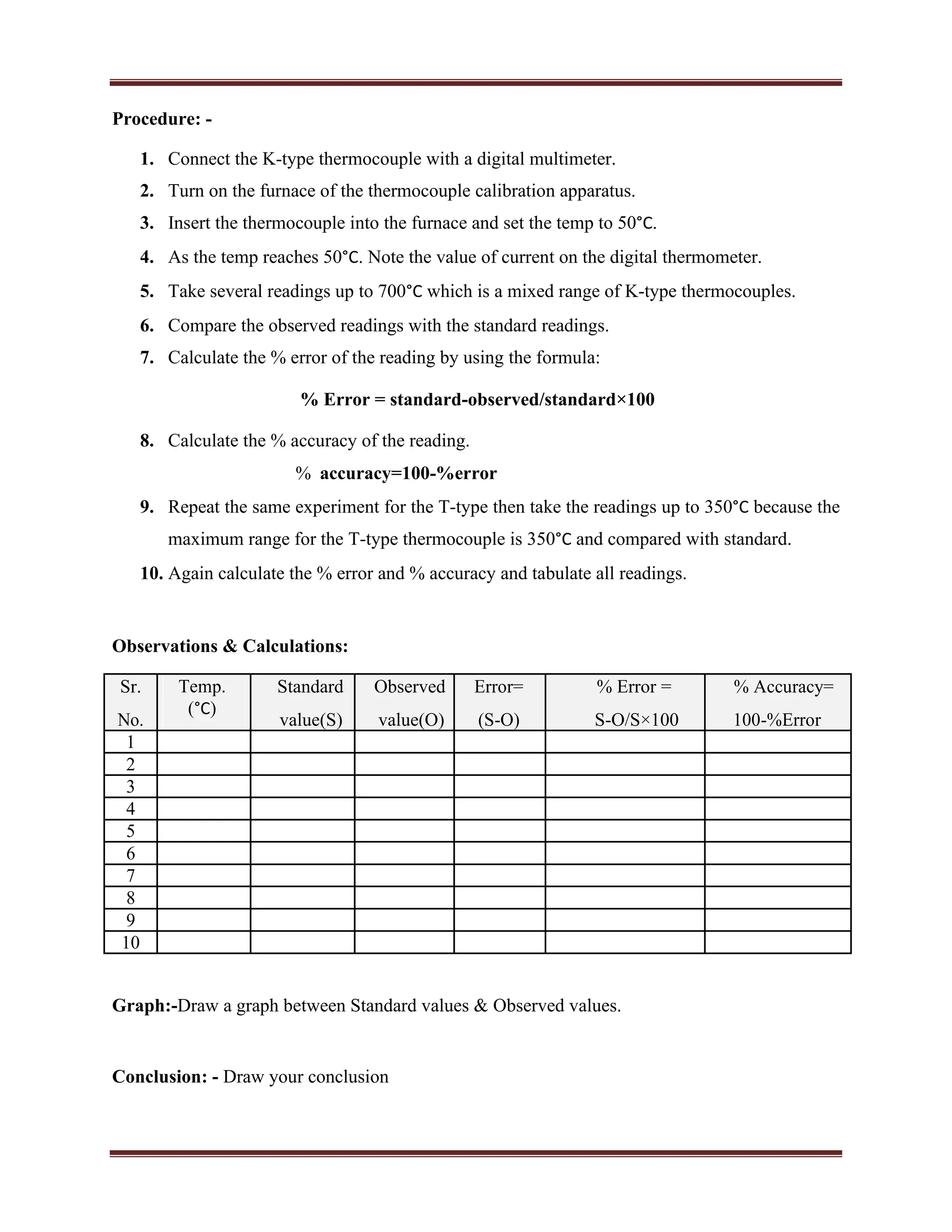
SlideShare a Scribd company logo
Instrumentation & Control (ME-2121)
LABORATORY MANUAL
INSTRUMENTATION
&
CONTROL
(ME-2121)
Prepared by:
ENGR. FAIZAN ASLAM
DEPARTMENT OF MATERIALS
NATIONAL TEXTILE UNIVERSITY
FAISALABAD - PAKISTAN
Overall Aims & Objectives of the Course:
The main objective of teaching this course is to give a general understanding of all the basic and
key concepts of instrumentation, necessary for process control. The primary aim of process control
is to maintain a process at the desired operating conditions, safely and efficiently, while satisfying
environmental and product quality requirements. A proper application of process control can
improve the safety and profitability of a process plant.
At the end of this lab course, students are expected to develop an ability to install, maintain and
calibrate the various instruments being used in different process industries. Furthermore, students
are expected to establish the ability to explain, discuss, and describe the principles & theories
related to the basic process control instrumentation, as well as, to analyze instrumentation diagrams
and design simple instrumentation control systems.
LABORATORY SCHEDULE
Experiment No. Title of Experiment
0 Laboratory Layout
1
To report the accuracy of the Bourdon pressure gauges by calibrating it
with the help of the Dead Weight Tester Apparatus.
2
To calibrate the Bourdon gauges by using Pressure Calibration Apparatus
and report its accuracy.
3
To calibrate the different types of thermocouples by using a Thermocouple
Calibration Apparatus.
4 Calibration of Thermocouples by using Multi-function Calibrator.
5
To examine & evaluate the behavior of the Open-loop System in Pressure
Control Station and control Pressure with two Solenoid valves.
To inspect the behavior of the Closed-loop System in the Pressure Control
Station
6
by manipulating the set point. Also, analyze & interpret the experimental
data for the response of disturbance on given System. (Solenoid valve#1
and solenoid valve#2)
Open-ended lab
To predict the behavior of the Closed-loop System in the Pressure Control
Station by manipulating the set point. Also, analyze & interpret the
experimental data for the response of disturbance in a given System.
(Motorized valve)
To examine & evaluate the behavior of the Open-loop System in Level
Control
8 Station and control the Level manually. Also, summarize the difficulties in
manual control.
To inspect the behavior of the Closed-loop System in the Level Control
Station by
9 manipulating the set point. Also, examine & interpret the experimental data
for the response of disturbance on a given System (Pump only)
To predict the behavior of the Closed-loop System in the Level Control
Station by
Open-ended lab manipulating the set point. Also, analyze & interpret the experimental data
for the response of disturbance on the given System. (Pump & Solenoid
valve)
To inspect the behavior of the Closed-loop System in the Level Control
Station by
11 manipulating the set point. Also, examine & interpret the experimental data
for the response of disturbance on the given System. (Motorized valve)
To examine the behavior of a Closed-loop System in a Flow Control Station
12 by manipulating the set point. Also, evaluate & interpret the experimental
data for the response of disturbance on given System.
To interpret the behavior of the Closed-loop System in Temperature Control
13 Station by manipulating the set point. Also, evaluate & interpret the
experimental data for the response of disturbance on a given System.
14
To determine the Time Constant of the mercury-bulb thermometer dipped in
an oil bath. Also, plot a graph b/w Y(t)/A and t.
Experiment No. 1
EXPERIMENT NO. 1
Objective: -
To report the accuracy of the Bourdon pressure gauge by calibrating it with the help of the Dead
Weight Tester apparatus.
Theory: -
A Dead Weight Tester apparatus uses known traceable weights to apply pressure to a fluid for
checking the accuracy of readings from a pressure gauge. There are three main components of this
device: a fluid (oil) that transmits the pressure, weight and piston used to apply pressure and a
connection port for the gauge to be calibrated.
The Dead Weight Tester also contains an oil reservoir and an adjusting piston or screw pump. The
reservoir accumulates oil displaced by the vertical piston during a calibration when a range of
accurately calibrated weights is used for a given gauge. The adjusting piston is used to make sure
that the vertical piston is freely floating on the oil.
Working Principle: -
A Dead Weight Tester consists of a pumping piston with a screw that presses it into the reservoir
containing a fluid like oil a primary piston that carries the dead weight (W) and the pressure gauge
to be calibrated as shown in the diagram. It works by loading the primary piston of cross-sectional
area (A) with the amount of weight (W) that corresponds to the desired calibration pressure
(P=W/A). The pumping piston then pressurizes the whole system by pressing more fluid into the
reservoir cylinder.
When the screw has turned the increase in fluid pressure is applied by both the gauge and the
weights. When the weights start to lift, the gauge pressure should be the same as the pressure
indicated by the weights.
Figure: Dead weight tester/apparatus
Procedure: -
1. Remove the piston from the unit.
2. Close valve V1 and open valve V2.
3. Fill the cylinder with oil.
4. Now close valve V2.
5. Put the piston back in the piston with V1 and V2 in a close position.
6. Read out pressure value on gauge and compare it with theoretical results.
7. Calculate the % Error & % Accuracy of Dead Weight Tester.
8. Repeat the experiment by adding weights.
Observations& Calculations:
Sr. Applied Applied Theoretical
Practical
%Error =
Area Pressure Error %Accuracy
No. Load Load Pressure
(m2
) (PP) =(PT- PP) T- P T =100-%Error
(kg) (N) (PT)(N/m2
) 2 (P P )/P ×100
(N/m )
1
2
3
4
5
Graph: -Draw a graph between Theoretical Pressure & Practical Pressure
Conclusion:- Draw your conclusion
.
Experiment No. 2
EXPERIMENT NO. 2
Objective:-
To calibrate the Bourdon gauges by using Pressure Calibration Apparatus and report its accuracy.
Theory:
The Bourdon gauge is a traditional and probably the most recognizable pressure measuring
instrument. It has a rotary scale and indicator needle. The dial is calibrated in both ordinary units
(degree of rotation) and engineering units of pressure.
Figure: Bourdon Pressure gauges
Working Principle:
The pressure of the entered fluid forces the hollow curved bourdon tube to straighten, turning the
gears and moving the needle.
Figure: Design and Construction
Usage Examples:
Simplicity & small size makes the bourdon gauge a popular pressure measuring device. It is used
for measuring pressure in liquids and gases of many different types of industries such as oil
exploration wells, refineries, petrochemical processing plants, hydraulic & pneumatic
installations, power stations, and wastewater operations, etc.
Advantages Disadvantages
1. Simple to use, safe, and inexpensive 1. Measurement of pressure at high
2. Can be used for a wide range of pressure, temperatures may cause deformation in the
from 0 to 7000 atm gauge, resulting in systematic errors
3. Can be used instead of manometers at
extreme pressures & temperatures
Questions to be asked by yourself:
1. Why do we calibrate the instruments?
2. Why it is necessary/important?
Procedure: -
1. Set the apparatus in operating conditions.
2. Switch on the apparatus.
3. Switch on the compressor.
4. Increased the Pressure in the storage tank.
5. Opened the valve of the process tank.
6. Set a value.
7. Then started depressurizing and note the readings for an interval of 10.
8. Tabulate the readings.
9. Calculate the values of pressure and compared them with standard values.
10. Draw the graph of pressurizing & depressurizing (b/w gauge pressure and standard
pressure).
Observations& Calculations:
Span=0-140psi
Sr.No. Standard Gauge
Error =(S-G)
% Error = % Accuracy=
Pressure (S) Pressure (G) S-G/S×100 100-%Error
1
2
3
4
5
6
7
8
9
10
Graph:- Draw a graph between Standard Pressure & Gauge Pressure
Conclusion: - Draw your conclusion
Experiment No. 3
EXPERIMENT NO. 3
Objective: -
To calibrate the different types of thermocouples by using the Thermocouple Calibration
Apparatus.
Apparatus: -
1. Thermocouples (K-type, T-type, etc.)
2. Connecting wires
3. Multi-meter
4. Calibration apparatus
Theory: -
A thermocouple has two electrical conductors made of different metals. The key requirement is
that the connection b/w the two conductors at both ends must form a good electrical connection.
A thermocouple measures the temperature difference between its two junctions. To measure the
temperature of one of the junctions, the temperature of the other junction must be known Voltage
differential measured at the output of the thermocouple is approximately proportional to the
temperature differential b/w the two points.
Vout ≈ K. (T1-T2)
The proportionality constant (K) is a function of thermocouple materials (not exactly a constant
that varies with temperature). The output voltage of the thermocouple is in the mV range and must
be amplified by an operational amplifier before it is used by a data-acquisition system.
Figure: A typical Thermocouple
Working Principle: -
The working principle of a thermocouple is stated as “when two dissimilar metal wires are
connected in a loop at two different temperatures a voltage potential will be generated and current
will flow through the loop circuit.”
Figure: Design and Construction of Thermocouple
Usage Examples:
Applications of Thermocouples may be found in heating systems (i.e. furnaces, boilers,
etc.) and cooling systems (i.e. chillers, refrigeration systems, etc.). Other examples include
reactors, heat exchangers, distillation columns, evaporators, kilns, absorbers, strippers, etc.
ADVANTAGES DISADVANTAGES
1. Simple to use, inexpensive & Accurate 1. Poor sensitivity to small temp changes
2. Rugged & Reliable
2. Temperature of reference junction required to be
maintained
3. Compact size
3. Small output voltage (mV) signal needs
amplification
4. Quick response as compared to RTD 4. Electromagnetic influence due to generation of
5. Wide temp range (-273°C to 2800°C) voltage in lead wires
Procedure: -
1. Connect the K-type thermocouple with a digital multimeter.
2. Turn on the furnace of the thermocouple calibration apparatus.
3. Insert the thermocouple into the furnace and set the temp to 50°C.
4. As the temp reaches 50°C. Note the value of current on the digital thermometer.
5. Take several readings up to 700°C which is a mixed range of K-type thermocouples.
6. Compare the observed readings with the standard readings.
7. Calculate the % error of the reading by using the formula:
% Error = standard-observed/standard×100
8. Calculate the % accuracy of the reading.
% accuracy=100-%error
9. Repeat the same experiment for the T-type then take the readings up to 350°C because the
maximum range for the T-type thermocouple is 350°C and compared with standard.
10. Again calculate the % error and % accuracy and tabulate all readings.
Observations & Calculations:
Sr. Temp.
(°C)
Standard Observed Error= % Error = % Accuracy=
No. value(S) value(O) (S-O) S-O/S×100 100-%Error
1
2
3
4
5
6
7
8
9
10
Graph:-Draw a graph between Standard values & Observed values.
Conclusion: - Draw your conclusion
Experiment No. 4
EXPERIMENT NO. 4
Objective: -
Calibration of Thermocouples by using Multi-function Calibrator.
Apparatus: -
1. Multi-Function Calibrator (tecpe-cl-325)
2. Digital Multi Meter (escort-172)
3. J and k type thermocouple
4. Connecting wires
5. DC battery
Theory: -
Multi Meter: -
A multi-meter also known as a VOM (Volt-Ohm Meter), is an electronic instrument that combines
several measurement functions in one unit. A typical multimeter would include basic features such
as the ability to measure voltage, current, and resistance.
Analog multi-meters use a micro-ammeter whose pointer
moves over a scale calibrated for all the different
measurements that can be made. Digital multi-meters (DMM)
display the measured value in numerals, and may also display
a bar of a length proportional to the quantity being measured.
Digital multi-meters are now far more common but Analog
multi-meters are still preferable in some cases, for example
when monitoring a rapidly varying value.
A Digital multimeter can be a hand-held device useful for
basic fault finding and field service work, or a bench
instrument that can measure to a very high degree of
accuracy. They can be used to troubleshoot electrical
problems in a wide array of industrial and household devices
such as electronic equipment, motor controls, domestic
appliances, power supplies, and wiring systems.
Fig: Digital multi-meter
Digital multi-meter Vs. Analog multimeter
Digital Multimeter Analog Multimeter
1. High cost 1. Less costly
2. Give the output in numerical form,
displayed 2. Give the output as a reading on a scale
on screen against a pointer
3. Have less uncertainty (about 0.5% or 3. Have greater uncertainty in the measurement
less) (about 3%)
4. Have a better range of measurements 4. Range of measurements is less
5. Calibrated automatically before every 5. Calibrated manually
measurement.
6. Most of the digital multi-meters have auto- 6. Manually set for the specific
ranging feature range of measurement
7. Can be operated by a trained person 7. Need the practice in taking good
measurements
Procedure:-
1. Connected the j-type thermocouple with a digital multimeter.
2. Set a digital multi-function unit on °C and digital multi-meter on mA.
3. Now enter the value of temp say about 50°C on the multi-function calibrator and got the
value of current in mA.
4. Take readings up to a higher temp range of j-type thermocouple which is 760C °C.
5. Now calculate the % error by using the formula.
% Error = standard reading-observation reading/standard reading
6. Calculate the % accuracy by using the formula.
% accuracy=100%- error
7. Repeat the same experiment for a t-type thermocouple and take readings up to 350°C
starting from 50°C.
8. Tabulate all the readings and note the variation in %age accuracy.
Observations and calculations: -
Temp.
Current from Standard
Observed
Sr. value(O) of %Error= %Accuracy=
digital multi- value(S) of Error(S-O)
No. (°C) current (S-O)/S×100 100-%error
meter (mA) current (mA)
(mA)
1
2
3
4
5
6
7
8
9
10
Graph:-Draw a graph between Standard values & Observed values of current.
Conclusion: - Draw your conclusion
.
Experiment No. 5
EXPERIMENT NO. 5
Objective:-
To examine & evaluate the behavior of the Open-loop System in the Pressure Control Station
and control Pressure with two Solenoid valves.
Objective:-
1) Study the behavior of the open loop control system on the pressure process station.
2) Report the difficulties in manual control.
Equipment:-
Pressure Process Station.
Theory:-
Open Loop Control System:
A system in which the output quantity has no effect on the process input quantity is called Open
Loop Control System.
A characteristic of the open-loop controller is that it does not use feedback to determine if its output
has achieved the desired goal of the input. This means that the system does not observe the output
of the processes that it is controlling. Consequently, a true Open Loop System cannot engage in
machine learning and also cannot correct any errors that it could make. It also may not compensate
for disturbances in the system.
Usage Examples:
A typical example would be a conventional washing machine, for which the length of machine
wash time is entirely dependent on the judgment and estimation of the human operator. Other
examples are an irrigation sprinkler system, Bread Toaster, an Automatic Tea/Coffee Maker,
Timer Based Clothes Drier, etc.
Advantages & Disadvantages of Open Loop Control System
Advantages Disadvantages
1. Simple in construction and design. 1. Inaccurate & unreliable.
2. Economical. 2. Effected on disturbance.
3. Easy to maintain.
3. Any change in output cannot be
corrected automatically.
4. Convenient to use as output is difficult to
measure.
Pressure transducer/transmitter: -
Working Principle: -
A pressure transducer is a transmitter that converts pressure into an electrical signal. One of
the most common of this kind is the strain-gauge which is a passive type resistance pressure
transducer, whose electrical resistance changes when it is stretched or compressed. It can be
attached to a pressure-sensing diaphragm and wired into a Wheatstone bridge configuration.
Pressure applied produces a deflection of the diaphragm which introduces strain to the gauge. This
strain will produce an electrical resistance change that is proportional to the applied pressure.
Figure: Pressure Transducer/Transmitter
Usage Examples:
Applications of Pressure Transducer/Transmitter may be found in Natural Gas Equipment
(Compressors and Dispensing Equipment), Power Plants (Piping Steam Pressure), Refrigeration,
Robotics (Factory Automated Equipment) & Transportation (Breaking, Compressors, Lifts, Air
Conditioning) etc.
Advantages & Disadvantages of Pressure transducer/transmitter
Advantages Disadvantages
1. They have good accuracy & stability 1. Their cost is moderate to high
2. They are compact, easy to install & 2. Wheatstone bridge is required to measure
simple to maintain the output of the strain gauge.
3. They possess a fast speed of response. 3. The bridge output voltage is also small and
amplification has to be carried out.
4. Available for a wide range of measurements 4. They require a constant voltage supply
Procedure: -
1. First of all, turned on the pressure process station.
2. Set the pressure range to say 60 psi. Then turned on the compressor. Now, turned off the
auto-mode of the solenoid valve and operated the solenoid valve.
3. Similarly, repeat this step and take at least five readings for the depressurized solenoid
valve.
4. Repeat the same experiment for the pressurized solenoid valve and take five readings for
pressurizing. Draw a graph between the set point and actual pressure and note the
difference between these values.
Observations & Calculations:-
For pressurized solenoid valve:
Sr. No. Actual pressure Set point pressure Pressure difference
(psi) (psi) (psi)
1
2
3
4
5
For depressurized solenoid valve:
Sr. No. Actual pressure Set point pressure Pressure difference
(psi) (psi) (psi)
1
2
3
4
5
Graph: - Draw a graph between Actual Pressure & Set Point Pressure.
Conclusion: - Draw your conclusion
Experiment No. 6
EXPERIMENT NO. 6
Objective:
To inspect the behavior of Closed-loop System in Pressure Control Station by manipulating the
set point. Also analyze & interpret the experimental data for the response of disturbance on given
System. (Solenoid valve#1 and solenoid valve#2)
Apparatus: -
Pressure Process Station.
Theory: -
Closed Loop Control System:
A system in which the output has an effect upon the process input quantity in such a manner as to
maintain the desired output value is called Closed Loop Control System.
Feedback is a special feature of a closed-loop control system. A closed loop control system
compares the output with the expected result or command status, and then it takes appropriate
control actions to adjust the input signal. Therefore, a closed loop system is always equipped with
a sensor, which is used to monitor the output and compare it with the expected result. The output
signal is fed back to the input to produce a new output. A well-designed feedback system can often
increase the accuracy of the output.
Figure: A closed-loop control system
Usage Examples:
Practical Examples of Closed Loop Control Systems are Automatic Electric Iron, Missile
Launched & Auto Tracked by Radar, An Air Conditioner and Cooling System in Car, etc.
Advantages & Disadvantages of Closed Loop Control System
Advantages Disadvantages
1. Accurate and Reliable 1. High Cost
2. Stable 2. Complicated Design
3. Affects disturbance and minimizes it 3. Require high maintenance
4. Facilitates automation
Procedure: - (solenoid valve 1 and solenoid valve 2)
1. Switch on the apparatus and then the compressor.
2. Turn the solenoid valve on in auto mode.
3. Set the solenoid valve 1 output as the primary output.
4. Set the solenoid valve 2 as the secondary output of the controller.
5. Set the controller on a closed loop and then give the set point to the controller.
6. Now give a set value to the controller.
7. Note the reading after some time until the fluctuations end.
8. Reset the value and not the readings.
9. Plot the graph between the time process variable.
Observations & Calculations: -
Sr. No. Actual pressure Set point pressure Pressure difference
(psi) (psi) (psi)
1
2
3
4
5
Graph: - Draw a graph between Actual Pressure & Set Point Pressure.
Conclusion: - Draw your conclusion
Experiment No. 7
EXPERIMENT NO. 7
Objective: -
To predict the behavior of the Closed-loop System in the Pressure Control Station by manipulating
the set point. Also, analyze & interpret the experimental data for the response of disturbance in a
given System. (Motorized valve)
Apparatus: -
Pressure Process Station.
Theory: -
Motor Operated Valve (MOV):
Motor Operated Valve (MOV) is an important item of the Plant & Piping system. These valves
are generally large and are used for different applications such as Pump discharge etc. Motor
Operated Valves are often called On-Off valves as the motors serve the purpose of fully opening
or fully closing valves in pipelines. For example, in cooling water lines, and process pipelines
where controlling of fluid is not required, motor-operated valves can be used to fully allow or fully
stop the fluid flow. These valves are not used for throttling purposes as they serve mainly ON-
OFF service applications.
Motor-operated valves can be of various types e.g. Gate/ Ball/ Butterfly etc. with actuator control.
The design of Motors and valves can be different. An electric motor is mounted on the valve and
geared to the valve stem so that when the motor operates the valve will open or close. For this
MOV, a motor operated with actuator control from the local panel or, from the control room is
required. There is a requirement for coordination among Piping-Electrical-Instrumentation-
Process engineers and vendors for the design and procurement of such motor-operated valves.
Figure: A typical motorized valve
Figure: Typical air-operated control valve
Figure: A pneumatic control valve
Types of Motor Operated Valves
The motorized control valve can be classified into three types. However, it must be noted that
the main application of motorized valves is for flow control and flow isolation.
Open/Close Valves: -
Used to automate manually open-close valves. Examples include pump discharge/suction
valves, boiler feed water isolation valves, drum vent valves, product line valves, etc.
Inching Valves: -
Used where some degree of control is required. Applications include reflux lines, boiler start-
up vents, boiler mainstream valves, etc.
Precision Flow Valves: -
In the inching valve, the motor operates in steps configured in the controller, e.g. 5%, 10%
opening steps. In precision flow valves, continuous control is enabled by the use of proper
feedback from the field to the controller which is not usually found in other motor-operated
valves. An example includes steam injection valve/water injection valve etc.
Advantages &Disadvantages of Motorized Valves
Advantages Disadvantages
1. Accurate & Reliable 1. Initial High cost
2. Fast Response
3. Require less maintenance 2. Need precise & accurate Motor to control
4. Can be used in hazardous locations where valve’s positions
The human-operator approach is
inaccessible.
Procedure: - (Motorized Valve)
1. Switch on the apparatus and then the compressor.
2. Turn the motorized valve on auto mode.
3. Set the motorized valve open as the primary output.
4. Set the motorized valve closed as the secondary output of the controller.
5. Set the controller on a closed loop and then give the set point to the controller.
6. Now give a set valve to the controller.
7. Note the reading after some time until the fluctuations end.
8. Reset the other set point and note the readings.
9. Plot the graph between the time process variable.
Observations & Calculations: -
Sr. No. Actual pressure Set point pressure Pressure difference
(psi) (psi) (psi)
1
2
3
4
5
Graph:-Draw a graph between Actual Pressure & Set Point Pressure.
Conclusion: - Draw your conclusion
.
Experiment No. 8
EXPERIMENT NO. 8
Objective: -
To examine & evaluate the behavior of the Open-loop System in the Level Control Station and
control the Level manually. Also, summarize the difficulties in manual control.
1) Study the behavior of the open loop control system on the level controller apparatus.
2) Control the level of fluid manually.
3) Report the difficulties in manual controls.
Equipment: -
Level Process Station.
Theory: -
Manual Control System:
A system that is totally Controlled or Manipulated by a human operator is called Manual Control
System.
Figure: A manual control valve system
Advantages & Disadvantages of Manual Control System
Advantages Disadvantages
1. Initial purchase cost is low 1. Inaccurate and Unreliable
2. Easy to handle and understand 2. Time-consuming
3. No need for electricity 3. Lack of security
4. Easy to construct and Maintain 4. It requires an operator for continuous
monitoring of a system
Differential Pressure (DP) Transmitter:-
Working Principle:-
Differential pressure transmitters measure the difference in pressure between two points. DP
transmitter converts the differential pressure of liquid into the level. This device uses two pressure
detectors. One is placed at the bottom of the vessel to make high pressure measurement. The other
sensor is placed in the vapor space for vessel pressure measurement. The following formula
indicates what factors influence its readings.
High-pressure measurement = Hydrostatic head + Vessel pressure
Advantages & Disadvantages of Differential Pressure Transmitter
Advantages Disadvantages
1. Poor sensitivity to small temp changes 1. Poor sensitivity to small temp changes
2. Temperature of reference junction required to 2. Temperature of reference junction required to be
be maintained maintained
3. Small output voltage (mV) signal needs 3. Small output voltage (mV) signal needs
amplification amplification
Procedure: -
1. First of all, turned on the level process station.
2. Then turned on the manual mode of the motorized valve to operate it manually.
3. Set the value for the level of fluid on the digital controller.
4. Open the valve of the controller and also turned on the motor and filled the fluid in the DP
cell more than the set value.
5. Now open the motorized valve, and removed the fluid out of the tank up to the set value of
fluid level.
6. There is a variation between the set value and the actual level.
7. Repeat the same steps and take almost 5 readings.
8. Tabulate all the readings and note the difference b/w actual and set levels.
9. Also, draw a graph b/w actual level and set values.
Observation & Calculation: -
Sr. No. The actual level of fluid (inches) Set point (inches) Difference
1
2
3
4
5
Graph:-Draw a graph between Actual Value & Set Point Value.
Conclusion: - Draw your conclusion
Experiment No. 9
EXPERIMENT NO. 9
Objective: -
To inspect the behavior of the Closed-loop System in the Level Control Station by manipulating
the set point. Also, examine & interpret the experimental data for the response of disturbance on a
given System (Pump only)
Apparatus: -
Level Process Station.
Theory: -
The Controller: -
It is an element in the process control loop, which evaluates any error of the measured variable
and initiates corrective action by changing the manipulated variable.
1. On/Off Control Action: -
It is the most basic type of control, which includes only two states/positions usually fully ON or
OFF. It is also known as two-position control. It’s simple, inexpensive & inherently reliable. It
offers relatively poor control. Rapid oscillations associated with it may result in equipment wear
which shortens its life.
2. Proportional (P) Controllers: -
The (P) controller shows a relatively high maximum overshoot, a long settling time as well as a
steady state error.
3. Integral (I) Controllers: -
The (I) controller has a higher maximum overshoot than the (P) controller due to the slowly starting
(I) behavior, but no steady-state error.
4. Derivative (D) Controllers: -
The (D) controller has less, maximum overshoot than the (P) controller and it has steady-state
error.
5. Proportional Integral (PI) Controllers: -
The (PI) controller fuses the properties of the (P) and (I) controllers. It shows a maximum
overshoot and settling time similar to the (P) controller but no steady-state error.
6. Proportional Derivative (PD) Controllers: -
The (PD) controller has a smaller maximum overshoot due to the faster D action. Also in this case
a steady state error is visible, which is smaller than in the case of the (P) controller.
7. Proportional Integral Derivative (PID) Controllers: -
The (PID) controller combines the properties of (PI) and (PD) controllers. It shows a smaller
maximum overshoot than the (PD) controller and has no steady-state error due to the (I)action.
The following are general rules that should be followed:
Flow Control requires Proportional and Integral. The derivative is not normally required.
Level Control uses Proportional and sometimes Integral, Derivative is not normally required.
Pressure Control requires Proportional and Integral; Derivative is normally not required. Temperature
Control uses Proportional, Integral, and derivatives usually with Integral set for a long time period.
Procedure: - (Pump only)
1. Switch on the apparatus and then pump.
2. Turn the pump on auto mode.
3. Set the pump output as the primary output.
4. Now select the ON/OFF controller.
5. Set the controller on a closed loop and then give the set point to the controller.
6. Now give a set value to the controller.
7. Note the reading after some time until the fluctuations end.
8. Reset the other set point and noted the readings.
9. Plot the graph between the time process variable.
Observations & Calculations:-
Set point = Inches Set point = Inches Set point = Inches
Sr. No. Time(sec) Indicated Time(sec) Indicated Time(sec) Indicated
Value Value Value
1
2
3
4
5
6
7
8
9
10
11
12
13
14
15
Graph:-Draw a graph between Time & Indicated Values.
Conclusion: - Draw your conclusion
Experiment No. 10
EXPERIMENT NO. 10
Objective: -
To predict the behavior of the Closed-loop System in Level Control Station by manipulating the
set point. Also, analyze & interpret the experimental data for the response of disturbance in a given
System. (Pump & Solenoid valve)
Apparatus: -
Level Process Station.
Theory: -
Centrifugal Pump: -
A centrifugal pump converts rotational energy, often from a motor, to energy in a moving fluid. A
portion of the energy goes into the kinetic energy of the fluid. Fluid enters axially through the eye
of the casing, is caught up in the impeller blades, and is whirled tangentially and radially outward
until it leaves through all circumferential parts of the impeller into the diffuser part of the casing.
The fluid gains both velocity and pressure while passing through the impeller. The doughnut-
shaped diffuser, or scroll, a section of the casing decelerates the flow and further increases the
pressure.
Figure: Construction of centrifugal pump
Usage Examples: -
Many different industries employ centrifugal pumps for different uses according to the industry.
For example, cryogenics use centrifugal pumps in extreme cold applications; dairy farmers use
centrifugal pumps to keep their product at the proper temperatures, hot and cold; electric utility
companies use centrifugal pumps, or turbines, to produce energy; food service, construction,
distillery, and automotive companies are a few more examples of industries that employee
centrifugal pumps for their many applications.
Advantages & Disadvantages of Centrifugal Pump
Advantages Disadvantages
1. Provide a continuous flow 1. Need Priming
2. Small in size and takes up little space for 2. Cannot be able to work high head.
installation.
3. Low price and need less maintenance
3. Long rotating shaft can cause leakage and
water wastage
4.Tough and sturdy because they don’t have
any sensitive part
5. No need of stepping because you can
4. Cannot deal with high viscous fluid.
connect them directly to a power source
6. Efficient to handle liquids.
7. Can be applied in industries to move out
acidic fluid
Solenoid Valve:
A solenoid valve is an electromechanically controlled valve. The valve features a solenoid, which
is an electric coil with a movable ferromagnetic core in its center. This core is called the plunger.
In the rest position, the plunger closes off a small orifice. An electric current through the coil
creates a magnetic field. The magnetic field exerts a force on the plunger. As a result, the plunger
is pulled toward the center of the coil so that the orifice opens. This is the basic principle that is
used to open and close solenoid valves.
Solenoid valves are the most frequently used control elements in fluidics. Their tasks are to shut
off, release and mix fluids. They are found in many application areas.
Usage Examples:
Some examples of solenoid valves include heating systems, compressed air technology, industrial
automation, swimming pools, sprinkler systems, washing machines, dental equipment, car wash
systems, irrigation systems, etc.
Advantages & Disadvantages of Solenoid Valves
Advantages Disadvantages
1. Fast And Safe Switching
1. Control signal must stay on during
operation
2. High Reliability
3. Long Service Life 2. Have only two positions fully open & fully
4. Low Power Consumption closed
5. Compact Design
Procedure: (Pump & Solenoid Valve)
1. Switch on the apparatus and then pump.
2. Turn the pump and solenoid valve on auto mode.
3. Set the pump output as the primary output.
4. Set the solenoid valve as the secondary output of the controller.
5. Set the controller on a closed loop and then give the set point to the controller.
6. Now give a set valve to the controller.
7. Note the reading after some time until the fluctuations ends.
8. Reset the other set point and note the readings.
9. Plot the graph between the time process variable.
Observations & Calculations:-
Set Point= Inches Set Point= Inches Set Point= Inches
Sr. No. Time(sec)
Indicated
Time(sec)
Indicated
Time(sec)
Indicated
Value Value Value
1
2
3
4
5
6
7
8
9
10
11
12
13
14
15
Graph:-Draw a graph between Time & Indicated Values.
Conclusion: - Draw your conclusion
Experiment No. 11
EXPERIMENT NO. 11
Objective: -
To inspect the behavior of the Closed-loop System in the Level Control Station by manipulating
the set point. Also, examine & interpret the experimental data for the response of disturbance in a
given System. (Motorized valve)
Apparatus: -
Level Process Station.
Theory: -
The Controller: -
It is an element in the process control loop, which evaluates any error of the measured variable
and initiates a corrective action by changing the manipulated variable.
1. On/Off Control Action: -
It is the most basic type of control, which includes only two states/positions usually fully ON or
OFF. It is also known as two-position control. It’s simple, inexpensive & inherently reliable. It
offers relatively poor control. Rapid oscillations associated with it may result in equipment wear–
shortens its life.
2. Proportional (P) Controllers: -
The (P) controller shows a relatively high maximum overshoot, a long settling time as well as a
steady state error.
3. Integral (I) Controllers: -
The (I) controller has a higher maximum overshoot than the (P) controller due to the slowly starting
(I) behavior, but no steady-state error.
4. Derivative (D) Controllers: -
The (D) controller has a smaller maximum overshoot than the (P) controller and it has a steady-
state error.
5. Proportional Integral (PI) Controllers: -
The (PI) controller fuses the properties of the (P) and (I) controllers. It shows a maximum
overshoot and settling time similar to the (P) controller but no steady-state error.
6. Proportional Derivative (PD) Controllers: -
The (PD) controller has a smaller maximum overshoot due to the faster D action. Also in this
case a steady state error is visible, which is smaller than in the case of the (P) controller.
7. Proportional Integral Derivative (PID) Controllers: -
The (PID) controller combines the properties of (PI) and (PD) controllers. It shows a smaller
maximum overshoot than the (PD) controller and has no steady-state error due to the (I) action.
The following are general rules that should be followed:
Flow Control requires Proportional and Integral. A derivative is not normally
required. Level Control uses Proportional and sometimes Integral, Derivative is not
normally
required.
Pressure Control requires Proportional and Integral; Derivative is normally not required.
Temperature Control uses Proportional, Integral, and Derivative usually with an Integral set
for a long period.
Procedure: (Motorized Valve)
1. Switch on the apparatus and then pump.
2. Turn on the pump in manual mode and set a flow rate.
3. Turn on the motorized valve in auto mode.
4. Set the motorized valve open as the primary output.
5. Set the motorized valve closed as the secondary output of the controller.
6. Set the controller on a closed loop and then give the set point to the controller.
7. Note the reading after some time until the fluctuations end.
8. Reset the other set point and note the readings.
9. Plot the graph between the time process variable.
Observations & Calculations: -
Set Point= Inches Set Point= Inches Set Point= Inches
Sr. No. Time(sec)
Indicated
Time(sec)
Indicated
Time(sec)
Indicated
value value value
1
2
3
4
5
6
7
8
9
10
11
12
13
14
15
Graph:-Draw a graph between Time & Indicated Values.
Conclusion: - Draw your conclusion
Experiment No. 12
EXPERIMENT NO. 12
Objective:-
To examine the behavior of the Closed-loop System in the Flow Control Station by manipulating
the set point. Also, evaluate & interpret the experimental data for the response of disturbance in a
given System.
Apparatus:-
Flow Process Station.
Theory:-
Turbine flow meter:-
Construction & Working Principle:-
It consists of a multi-bladed rotor (turbine wheel) which is mounted at right angles to the axis of
flowing fluid. The rotor is free to rotate about its axis. The speed of the rotor is directly proportional
to the fluid velocity. The speed of rotation is monitored by a magnetic-pickup coil which consists
of a permanent magnet. The turbine blades are made of magnetic material. As the fluid flows and
each blade passes by the coil, the magnetic flux through the coil changes, causing a voltage pulse.
A sensor measures the pulse rate which is a measure of the flow rate.
Figure: Construction of a turbine-type flow meter
Usage Examples: -
As an important application of the turbine meter is in the petrochemical industries, where gas/oil
mixtures are common, special procedures are being developed to avoid such large measurement
errors. Turbine flow meters are also used to measure the velocity of liquids, gases, and vapors in
pipes, such as hydrocarbons, chemicals, water, cryogenic liquids, air, and industrial gases.
Advantages & Disadvantages Turbine Flow meter
Advantages Disadvantages
1. Turbine flow meters are accurate with good flow 1. They are costly.
operating & temperature ranges.
2. It provides excellent repeatability & range ability. 2. Their use is limited to clean fluids such
3. It allows fairly low-pressure drops. as water & gasoline etc. They are not
4. It is easy to install & maintain. suitable for slurry applications.
Procedure: (Motorized regulator valve)
1. Switch on the apparatus.
2. Turn on the pump in manual mode and set a flow rate.
3. Turn on the motorized valve in auto mode.
4. Set the motorized valve open as the primary output.
5. Set the motorized valve closed as the secondary output of the controller.
6. Set the controller on a closed loop and then give the set point to the controller.
7. Note the reading after some time until the fluctuations end.
8. Reset the other set point and note the readings.
9. Plot the graph between the time process variable.
Observations and Calculations:-
Sr. No.
Frequency Set Value Present Value Difference Time
(Hz) (LPM) (LPM) (LPM) (sec)
1
2
3
4
5
6
7
8
9
10
Graph: - Draw a graph between Set Values & Present values.
Conclusion: - Draw your conclusion
Experiment No. 13
EXPERIMENT NO. 13
Objective: -
To interpret the behavior of the Closed-loop System in the Temperature Control Station by
manipulating the set point. Also, evaluate & interpret the experimental data for the response of
disturbance in a given System.
Apparatus: -
Temperature Process Station.
Theory:
To accurately control process temperature without an extensive operator, a temperature control
system relies upon a controller which accepts a temperature sensor such as a thermocouple as input
it compasses the actual temperature to the desired control temperature or set point and provides an
output to a control element. The controller is one part of the entry control system and the whole
system should be analyzed in selecting the proper controller.
Procedure: -
1. First of all, assure that all valves installed on the trainer are open.
2. Then turn on the pump and heater.
3. Set the controller into an automatic mode of operation.
4. Set the point at 40o
C and note the upper and lower limit of indicating temperature.
5. Repeat the procedure for 45°C, 50°C, 55°C, and 60°C.
Observations and Calculations:
Sr. No. Set Valve Present Valve Difference Time
(°C) (°C) (°C) (sec)
1
2
3
4
5
Graph: - Draw a graph between Set Values (°C) & Present values (°C).
Conclusion: - Draw your conclusion
Experiment No. 14
EXPERIMENT NO. 14
Objective: -
To calculate the Time Constant of the mercury-bulb thermometer dipped in an oil bath. Also,
plot a
graph b/w Y(t)/A and t.
Apparatus: -
1. Thermometer
2. Oil bath
Theory:
Time constant:
The time constant can be defined as the time required to
respond
63.3% of its output signal when subjected to a step change.
The step change can be either an increase or decrease in the
the parameter being measured the time constant depends on
airflow over the sensor.
There is no big advantage in using a thermometer with a very
small time constant. In many applications, it is necessary to
make measuring with time in order. To do this, we have to
know how to measurement system being used will respond to such
inputs.
Response:
The dynamic response of a temp measuring device can be modeled
as a first-order system. The first-order dynamic response is
characterized by one parameter “t” the time constant of a temp.
Working Principle of mercury bulb thermometer:
A thermometer works on the Thermal Expansion Principle which
states that the dimensions of all substances, whether solids, liquids,
or gases, change with temperature.
In a Thermometer, fluid is contained within a bulb and a capillary
tube. As the temperature rises, the fluid expands along the capillary
tube and the meniscus level is read against a calibrated scale etched
on the tube. The fluid used is usually either mercury or colored
alcohol.
Procedure:-
1. First of all pour 150 ml of lube oil into a beaker and placed the beaker on the heating surface.
2. Then start to heat the lube oil to 120°C.
3. Stopped heating when temp adore reaches 120°C.
4. Then in this way tabulated the result and plotted the graph.
Observations and Calculations:
Y=1200C (max temp) A=Y-room temp τ =mc/h.A
Sr. No. Time
(sec)
Temp 0C
(Ys)
Y(t)=Y-Ys Y(t)/A τ t/ τ
1
2
3
4
5
6
7
8
9
10
11
12
13
14
15
Graph: - Draw a graph between Set Values & Present values.
Conclusion: - Draw your conclusion

More Related Content

Similar to Instrumentation & Control Lab Manual.pdf

Shilpa ppt thermal plant copy
Shilpa ppt thermal plant   copyShilpa ppt thermal plant   copy
Shilpa ppt thermal plant copyShilpa Shukla
 
Power plant instrumentation
Power plant instrumentationPower plant instrumentation
Power plant instrumentation
T.SWAROOP KUMAR
 
Thermal plant instrumentation and control
Thermal plant instrumentation and controlThermal plant instrumentation and control
Thermal plant instrumentation and control
Shilpa Shukla
 
Dead weight piston gauge
Dead weight piston gaugeDead weight piston gauge
Dead weight piston gauge
Muhammed Fuad Al-Barznji
 
Control system-lab
Control system-labControl system-lab
Control system-lab
UdayKumar130463
 
DSC
DSCDSC
Venturi and orificemeter - Ed Ryan Ruales
Venturi and orificemeter - Ed Ryan RualesVenturi and orificemeter - Ed Ryan Ruales
Venturi and orificemeter - Ed Ryan Ruales
Ed Ryan Ruales
 
Water Temperature
Water TemperatureWater Temperature
Water TemperatureTheju Paul
 
Automated process control systems
Automated process control systemsAutomated process control systems
Automated process control systems
Shine Thenu
 
DEEP4.pdf
DEEP4.pdfDEEP4.pdf
DEEP4.pdf
rajvarya
 
Liquid Insulation Dissipation factor and Dielectric Factor Measurement Unit
Liquid Insulation Dissipation factor and Dielectric Factor Measurement UnitLiquid Insulation Dissipation factor and Dielectric Factor Measurement Unit
Liquid Insulation Dissipation factor and Dielectric Factor Measurement Unit
NadiiaHubar
 
Instrumentation Lab - Final.pptx
Instrumentation Lab - Final.pptxInstrumentation Lab - Final.pptx
Instrumentation Lab - Final.pptx
KannanRamaraj1
 
Hydraulic Hose Leak Testing (Test Rig is Pneumatic Hydraulic).pptx
Hydraulic Hose Leak Testing  (Test Rig is Pneumatic Hydraulic).pptxHydraulic Hose Leak Testing  (Test Rig is Pneumatic Hydraulic).pptx
Hydraulic Hose Leak Testing (Test Rig is Pneumatic Hydraulic).pptx
Neometrix_Engineering_Pvt_Ltd
 
Over all pressure of Fluid flow
Over all pressure of Fluid flowOver all pressure of Fluid flow
Over all pressure of Fluid flow
Aree Salah
 
ddc_controls_part_1_pnwd-sa-883dddds4.pdf
ddc_controls_part_1_pnwd-sa-883dddds4.pdfddc_controls_part_1_pnwd-sa-883dddds4.pdf
ddc_controls_part_1_pnwd-sa-883dddds4.pdf
nqmanuntag
 
MTCB lab manual.docx Maintenance of transformer and Circuit Breaker B
MTCB lab manual.docx   Maintenance of transformer and Circuit Breaker BMTCB lab manual.docx   Maintenance of transformer and Circuit Breaker B
MTCB lab manual.docx Maintenance of transformer and Circuit Breaker B
parulmp07
 
محاضرة 5
محاضرة 5محاضرة 5
محاضرة 5
ssuserd3a9b4
 
Chapter 55 Computer Sensors
Chapter 55 Computer SensorsChapter 55 Computer Sensors
Chapter 55 Computer Sensorsmcfalltj
 
INSTRUMENTATION AND PROCESS CONTROL - BOILER CONTROL
INSTRUMENTATION AND PROCESS CONTROL - BOILER CONTROLINSTRUMENTATION AND PROCESS CONTROL - BOILER CONTROL
INSTRUMENTATION AND PROCESS CONTROL - BOILER CONTROLno suhaila
 

Similar to Instrumentation & Control Lab Manual.pdf (20)

Shilpa ppt thermal plant copy
Shilpa ppt thermal plant   copyShilpa ppt thermal plant   copy
Shilpa ppt thermal plant copy
 
Power plant instrumentation
Power plant instrumentationPower plant instrumentation
Power plant instrumentation
 
Thermal plant instrumentation and control
Thermal plant instrumentation and controlThermal plant instrumentation and control
Thermal plant instrumentation and control
 
Dead weight piston gauge
Dead weight piston gaugeDead weight piston gauge
Dead weight piston gauge
 
Control system-lab
Control system-labControl system-lab
Control system-lab
 
DSC
DSCDSC
DSC
 
Venturi and orificemeter - Ed Ryan Ruales
Venturi and orificemeter - Ed Ryan RualesVenturi and orificemeter - Ed Ryan Ruales
Venturi and orificemeter - Ed Ryan Ruales
 
Water Temperature
Water TemperatureWater Temperature
Water Temperature
 
Automated process control systems
Automated process control systemsAutomated process control systems
Automated process control systems
 
DEEP4.pdf
DEEP4.pdfDEEP4.pdf
DEEP4.pdf
 
Liquid Insulation Dissipation factor and Dielectric Factor Measurement Unit
Liquid Insulation Dissipation factor and Dielectric Factor Measurement UnitLiquid Insulation Dissipation factor and Dielectric Factor Measurement Unit
Liquid Insulation Dissipation factor and Dielectric Factor Measurement Unit
 
Instrumentation Lab - Final.pptx
Instrumentation Lab - Final.pptxInstrumentation Lab - Final.pptx
Instrumentation Lab - Final.pptx
 
Hydraulic Hose Leak Testing (Test Rig is Pneumatic Hydraulic).pptx
Hydraulic Hose Leak Testing  (Test Rig is Pneumatic Hydraulic).pptxHydraulic Hose Leak Testing  (Test Rig is Pneumatic Hydraulic).pptx
Hydraulic Hose Leak Testing (Test Rig is Pneumatic Hydraulic).pptx
 
Over all pressure of Fluid flow
Over all pressure of Fluid flowOver all pressure of Fluid flow
Over all pressure of Fluid flow
 
ddc_controls_part_1_pnwd-sa-883dddds4.pdf
ddc_controls_part_1_pnwd-sa-883dddds4.pdfddc_controls_part_1_pnwd-sa-883dddds4.pdf
ddc_controls_part_1_pnwd-sa-883dddds4.pdf
 
MTCB lab manual.docx Maintenance of transformer and Circuit Breaker B
MTCB lab manual.docx   Maintenance of transformer and Circuit Breaker BMTCB lab manual.docx   Maintenance of transformer and Circuit Breaker B
MTCB lab manual.docx Maintenance of transformer and Circuit Breaker B
 
Lab manual.pptx
Lab manual.pptxLab manual.pptx
Lab manual.pptx
 
محاضرة 5
محاضرة 5محاضرة 5
محاضرة 5
 
Chapter 55 Computer Sensors
Chapter 55 Computer SensorsChapter 55 Computer Sensors
Chapter 55 Computer Sensors
 
INSTRUMENTATION AND PROCESS CONTROL - BOILER CONTROL
INSTRUMENTATION AND PROCESS CONTROL - BOILER CONTROLINSTRUMENTATION AND PROCESS CONTROL - BOILER CONTROL
INSTRUMENTATION AND PROCESS CONTROL - BOILER CONTROL
 

More from NTU Faisalabad

TE-3113-7.pdf mechanics of fibrous Structure slides
TE-3113-7.pdf mechanics of fibrous Structure slidesTE-3113-7.pdf mechanics of fibrous Structure slides
TE-3113-7.pdf mechanics of fibrous Structure slides
NTU Faisalabad
 
TE-3113-1.pdf
TE-3113-1.pdfTE-3113-1.pdf
TE-3113-1.pdf
NTU Faisalabad
 
Instrumentation and Control slide-3.pdf
Instrumentation and Control slide-3.pdfInstrumentation and Control slide-3.pdf
Instrumentation and Control slide-3.pdf
NTU Faisalabad
 
TE-3113-2.pdf
TE-3113-2.pdfTE-3113-2.pdf
TE-3113-2.pdf
NTU Faisalabad
 
The Rieter Manual of Spinning ll textilestudycenter.com ll V-3(Spinning Prep...
 The Rieter Manual of Spinning ll textilestudycenter.com ll V-3(Spinning Prep... The Rieter Manual of Spinning ll textilestudycenter.com ll V-3(Spinning Prep...
The Rieter Manual of Spinning ll textilestudycenter.com ll V-3(Spinning Prep...
NTU Faisalabad
 
Lec 19-21 Polymer Blends & Additives.pdf
Lec 19-21 Polymer Blends & Additives.pdfLec 19-21 Polymer Blends & Additives.pdf
Lec 19-21 Polymer Blends & Additives.pdf
NTU Faisalabad
 
Lec 30-33_Polymer Processing.pdf
Lec 30-33_Polymer Processing.pdfLec 30-33_Polymer Processing.pdf
Lec 30-33_Polymer Processing.pdf
NTU Faisalabad
 
Lec 25-29 Polymer Rheology.pdf
Lec 25-29 Polymer Rheology.pdfLec 25-29 Polymer Rheology.pdf
Lec 25-29 Polymer Rheology.pdf
NTU Faisalabad
 
Lec 25-29 Polymer Rheology.pdf
Lec 25-29 Polymer Rheology.pdfLec 25-29 Polymer Rheology.pdf
Lec 25-29 Polymer Rheology.pdf
NTU Faisalabad
 
8. YM-2012 Blow room - 8.pdf
8. YM-2012 Blow room - 8.pdf8. YM-2012 Blow room - 8.pdf
8. YM-2012 Blow room - 8.pdf
NTU Faisalabad
 
7. YM-2012 Blow room - 7.pdf
7. YM-2012 Blow room - 7.pdf7. YM-2012 Blow room - 7.pdf
7. YM-2012 Blow room - 7.pdf
NTU Faisalabad
 
6. YM-2012 Blow room - 6.pdf
6. YM-2012 Blow room - 6.pdf6. YM-2012 Blow room - 6.pdf
6. YM-2012 Blow room - 6.pdf
NTU Faisalabad
 
11. YM-2012 Basic action on card.pdf
11. YM-2012 Basic action on card.pdf11. YM-2012 Basic action on card.pdf
11. YM-2012 Basic action on card.pdf
NTU Faisalabad
 
10. YM-2012 Card objectives n working principle.pdf
10. YM-2012 Card objectives n working principle.pdf10. YM-2012 Card objectives n working principle.pdf
10. YM-2012 Card objectives n working principle.pdf
NTU Faisalabad
 
9. YM-2012 Card feed.pdf
9. YM-2012 Card feed.pdf9. YM-2012 Card feed.pdf
9. YM-2012 Card feed.pdf
NTU Faisalabad
 
GM NTU W10-1.pptx
GM NTU W10-1.pptxGM NTU W10-1.pptx
GM NTU W10-1.pptx
NTU Faisalabad
 
GM NTU W8-1.pptx
GM NTU W8-1.pptxGM NTU W8-1.pptx
GM NTU W8-1.pptx
NTU Faisalabad
 
Week-12(ph-1002).pptx
Week-12(ph-1002).pptxWeek-12(ph-1002).pptx
Week-12(ph-1002).pptx
NTU Faisalabad
 

More from NTU Faisalabad (20)

TE-3113-7.pdf mechanics of fibrous Structure slides
TE-3113-7.pdf mechanics of fibrous Structure slidesTE-3113-7.pdf mechanics of fibrous Structure slides
TE-3113-7.pdf mechanics of fibrous Structure slides
 
TE-3113-1.pdf
TE-3113-1.pdfTE-3113-1.pdf
TE-3113-1.pdf
 
Instrumentation and Control slide-3.pdf
Instrumentation and Control slide-3.pdfInstrumentation and Control slide-3.pdf
Instrumentation and Control slide-3.pdf
 
TE-3113-2.pdf
TE-3113-2.pdfTE-3113-2.pdf
TE-3113-2.pdf
 
The Rieter Manual of Spinning ll textilestudycenter.com ll V-3(Spinning Prep...
 The Rieter Manual of Spinning ll textilestudycenter.com ll V-3(Spinning Prep... The Rieter Manual of Spinning ll textilestudycenter.com ll V-3(Spinning Prep...
The Rieter Manual of Spinning ll textilestudycenter.com ll V-3(Spinning Prep...
 
Lec 19-21 Polymer Blends & Additives.pdf
Lec 19-21 Polymer Blends & Additives.pdfLec 19-21 Polymer Blends & Additives.pdf
Lec 19-21 Polymer Blends & Additives.pdf
 
Lec 30-33_Polymer Processing.pdf
Lec 30-33_Polymer Processing.pdfLec 30-33_Polymer Processing.pdf
Lec 30-33_Polymer Processing.pdf
 
Lec 25-29 Polymer Rheology.pdf
Lec 25-29 Polymer Rheology.pdfLec 25-29 Polymer Rheology.pdf
Lec 25-29 Polymer Rheology.pdf
 
Lec 25-29 Polymer Rheology.pdf
Lec 25-29 Polymer Rheology.pdfLec 25-29 Polymer Rheology.pdf
Lec 25-29 Polymer Rheology.pdf
 
8. YM-2012 Blow room - 8.pdf
8. YM-2012 Blow room - 8.pdf8. YM-2012 Blow room - 8.pdf
8. YM-2012 Blow room - 8.pdf
 
7. YM-2012 Blow room - 7.pdf
7. YM-2012 Blow room - 7.pdf7. YM-2012 Blow room - 7.pdf
7. YM-2012 Blow room - 7.pdf
 
6. YM-2012 Blow room - 6.pdf
6. YM-2012 Blow room - 6.pdf6. YM-2012 Blow room - 6.pdf
6. YM-2012 Blow room - 6.pdf
 
11. YM-2012 Basic action on card.pdf
11. YM-2012 Basic action on card.pdf11. YM-2012 Basic action on card.pdf
11. YM-2012 Basic action on card.pdf
 
10. YM-2012 Card objectives n working principle.pdf
10. YM-2012 Card objectives n working principle.pdf10. YM-2012 Card objectives n working principle.pdf
10. YM-2012 Card objectives n working principle.pdf
 
9. YM-2012 Card feed.pdf
9. YM-2012 Card feed.pdf9. YM-2012 Card feed.pdf
9. YM-2012 Card feed.pdf
 
GM NTU W10-1.pptx
GM NTU W10-1.pptxGM NTU W10-1.pptx
GM NTU W10-1.pptx
 
GM NTU W8-1.pptx
GM NTU W8-1.pptxGM NTU W8-1.pptx
GM NTU W8-1.pptx
 
Week-12(ph-1002).pptx
Week-12(ph-1002).pptxWeek-12(ph-1002).pptx
Week-12(ph-1002).pptx
 
Week-11.pptx
Week-11.pptxWeek-11.pptx
Week-11.pptx
 
Week-10.pptx
Week-10.pptxWeek-10.pptx
Week-10.pptx
 

Recently uploaded

Governing Equations for Fundamental Aerodynamics_Anderson2010.pdf
Governing Equations for Fundamental Aerodynamics_Anderson2010.pdfGoverning Equations for Fundamental Aerodynamics_Anderson2010.pdf
Governing Equations for Fundamental Aerodynamics_Anderson2010.pdf
WENKENLI1
 
ML for identifying fraud using open blockchain data.pptx
ML for identifying fraud using open blockchain data.pptxML for identifying fraud using open blockchain data.pptx
ML for identifying fraud using open blockchain data.pptx
Vijay Dialani, PhD
 
Gen AI Study Jams _ For the GDSC Leads in India.pdf
Gen AI Study Jams _ For the GDSC Leads in India.pdfGen AI Study Jams _ For the GDSC Leads in India.pdf
Gen AI Study Jams _ For the GDSC Leads in India.pdf
gdsczhcet
 
Heap Sort (SS).ppt FOR ENGINEERING GRADUATES, BCA, MCA, MTECH, BSC STUDENTS
Heap Sort (SS).ppt FOR ENGINEERING GRADUATES, BCA, MCA, MTECH, BSC STUDENTSHeap Sort (SS).ppt FOR ENGINEERING GRADUATES, BCA, MCA, MTECH, BSC STUDENTS
Heap Sort (SS).ppt FOR ENGINEERING GRADUATES, BCA, MCA, MTECH, BSC STUDENTS
Soumen Santra
 
Forklift Classes Overview by Intella Parts
Forklift Classes Overview by Intella PartsForklift Classes Overview by Intella Parts
Forklift Classes Overview by Intella Parts
Intella Parts
 
Water Industry Process Automation and Control Monthly - May 2024.pdf
Water Industry Process Automation and Control Monthly - May 2024.pdfWater Industry Process Automation and Control Monthly - May 2024.pdf
Water Industry Process Automation and Control Monthly - May 2024.pdf
Water Industry Process Automation & Control
 
HYDROPOWER - Hydroelectric power generation
HYDROPOWER - Hydroelectric power generationHYDROPOWER - Hydroelectric power generation
HYDROPOWER - Hydroelectric power generation
Robbie Edward Sayers
 
Tutorial for 16S rRNA Gene Analysis with QIIME2.pdf
Tutorial for 16S rRNA Gene Analysis with QIIME2.pdfTutorial for 16S rRNA Gene Analysis with QIIME2.pdf
Tutorial for 16S rRNA Gene Analysis with QIIME2.pdf
aqil azizi
 
Railway Signalling Principles Edition 3.pdf
Railway Signalling Principles Edition 3.pdfRailway Signalling Principles Edition 3.pdf
Railway Signalling Principles Edition 3.pdf
TeeVichai
 
DfMAy 2024 - key insights and contributions
DfMAy 2024 - key insights and contributionsDfMAy 2024 - key insights and contributions
DfMAy 2024 - key insights and contributions
gestioneergodomus
 
space technology lecture notes on satellite
space technology lecture notes on satellitespace technology lecture notes on satellite
space technology lecture notes on satellite
ongomchris
 
一比一原版(UofT毕业证)多伦多大学毕业证成绩单如何办理
一比一原版(UofT毕业证)多伦多大学毕业证成绩单如何办理一比一原版(UofT毕业证)多伦多大学毕业证成绩单如何办理
一比一原版(UofT毕业证)多伦多大学毕业证成绩单如何办理
ydteq
 
Final project report on grocery store management system..pdf
Final project report on grocery store management system..pdfFinal project report on grocery store management system..pdf
Final project report on grocery store management system..pdf
Kamal Acharya
 
road safety engineering r s e unit 3.pdf
road safety engineering  r s e unit 3.pdfroad safety engineering  r s e unit 3.pdf
road safety engineering r s e unit 3.pdf
VENKATESHvenky89705
 
NO1 Uk best vashikaran specialist in delhi vashikaran baba near me online vas...
NO1 Uk best vashikaran specialist in delhi vashikaran baba near me online vas...NO1 Uk best vashikaran specialist in delhi vashikaran baba near me online vas...
NO1 Uk best vashikaran specialist in delhi vashikaran baba near me online vas...
Amil Baba Dawood bangali
 
NUMERICAL SIMULATIONS OF HEAT AND MASS TRANSFER IN CONDENSING HEAT EXCHANGERS...
NUMERICAL SIMULATIONS OF HEAT AND MASS TRANSFER IN CONDENSING HEAT EXCHANGERS...NUMERICAL SIMULATIONS OF HEAT AND MASS TRANSFER IN CONDENSING HEAT EXCHANGERS...
NUMERICAL SIMULATIONS OF HEAT AND MASS TRANSFER IN CONDENSING HEAT EXCHANGERS...
ssuser7dcef0
 
CME397 Surface Engineering- Professional Elective
CME397 Surface Engineering- Professional ElectiveCME397 Surface Engineering- Professional Elective
CME397 Surface Engineering- Professional Elective
karthi keyan
 
Fundamentals of Electric Drives and its applications.pptx
Fundamentals of Electric Drives and its applications.pptxFundamentals of Electric Drives and its applications.pptx
Fundamentals of Electric Drives and its applications.pptx
manasideore6
 
Sachpazis:Terzaghi Bearing Capacity Estimation in simple terms with Calculati...
Sachpazis:Terzaghi Bearing Capacity Estimation in simple terms with Calculati...Sachpazis:Terzaghi Bearing Capacity Estimation in simple terms with Calculati...
Sachpazis:Terzaghi Bearing Capacity Estimation in simple terms with Calculati...
Dr.Costas Sachpazis
 
Top 10 Oil and Gas Projects in Saudi Arabia 2024.pdf
Top 10 Oil and Gas Projects in Saudi Arabia 2024.pdfTop 10 Oil and Gas Projects in Saudi Arabia 2024.pdf
Top 10 Oil and Gas Projects in Saudi Arabia 2024.pdf
Teleport Manpower Consultant
 

Recently uploaded (20)

Governing Equations for Fundamental Aerodynamics_Anderson2010.pdf
Governing Equations for Fundamental Aerodynamics_Anderson2010.pdfGoverning Equations for Fundamental Aerodynamics_Anderson2010.pdf
Governing Equations for Fundamental Aerodynamics_Anderson2010.pdf
 
ML for identifying fraud using open blockchain data.pptx
ML for identifying fraud using open blockchain data.pptxML for identifying fraud using open blockchain data.pptx
ML for identifying fraud using open blockchain data.pptx
 
Gen AI Study Jams _ For the GDSC Leads in India.pdf
Gen AI Study Jams _ For the GDSC Leads in India.pdfGen AI Study Jams _ For the GDSC Leads in India.pdf
Gen AI Study Jams _ For the GDSC Leads in India.pdf
 
Heap Sort (SS).ppt FOR ENGINEERING GRADUATES, BCA, MCA, MTECH, BSC STUDENTS
Heap Sort (SS).ppt FOR ENGINEERING GRADUATES, BCA, MCA, MTECH, BSC STUDENTSHeap Sort (SS).ppt FOR ENGINEERING GRADUATES, BCA, MCA, MTECH, BSC STUDENTS
Heap Sort (SS).ppt FOR ENGINEERING GRADUATES, BCA, MCA, MTECH, BSC STUDENTS
 
Forklift Classes Overview by Intella Parts
Forklift Classes Overview by Intella PartsForklift Classes Overview by Intella Parts
Forklift Classes Overview by Intella Parts
 
Water Industry Process Automation and Control Monthly - May 2024.pdf
Water Industry Process Automation and Control Monthly - May 2024.pdfWater Industry Process Automation and Control Monthly - May 2024.pdf
Water Industry Process Automation and Control Monthly - May 2024.pdf
 
HYDROPOWER - Hydroelectric power generation
HYDROPOWER - Hydroelectric power generationHYDROPOWER - Hydroelectric power generation
HYDROPOWER - Hydroelectric power generation
 
Tutorial for 16S rRNA Gene Analysis with QIIME2.pdf
Tutorial for 16S rRNA Gene Analysis with QIIME2.pdfTutorial for 16S rRNA Gene Analysis with QIIME2.pdf
Tutorial for 16S rRNA Gene Analysis with QIIME2.pdf
 
Railway Signalling Principles Edition 3.pdf
Railway Signalling Principles Edition 3.pdfRailway Signalling Principles Edition 3.pdf
Railway Signalling Principles Edition 3.pdf
 
DfMAy 2024 - key insights and contributions
DfMAy 2024 - key insights and contributionsDfMAy 2024 - key insights and contributions
DfMAy 2024 - key insights and contributions
 
space technology lecture notes on satellite
space technology lecture notes on satellitespace technology lecture notes on satellite
space technology lecture notes on satellite
 
一比一原版(UofT毕业证)多伦多大学毕业证成绩单如何办理
一比一原版(UofT毕业证)多伦多大学毕业证成绩单如何办理一比一原版(UofT毕业证)多伦多大学毕业证成绩单如何办理
一比一原版(UofT毕业证)多伦多大学毕业证成绩单如何办理
 
Final project report on grocery store management system..pdf
Final project report on grocery store management system..pdfFinal project report on grocery store management system..pdf
Final project report on grocery store management system..pdf
 
road safety engineering r s e unit 3.pdf
road safety engineering  r s e unit 3.pdfroad safety engineering  r s e unit 3.pdf
road safety engineering r s e unit 3.pdf
 
NO1 Uk best vashikaran specialist in delhi vashikaran baba near me online vas...
NO1 Uk best vashikaran specialist in delhi vashikaran baba near me online vas...NO1 Uk best vashikaran specialist in delhi vashikaran baba near me online vas...
NO1 Uk best vashikaran specialist in delhi vashikaran baba near me online vas...
 
NUMERICAL SIMULATIONS OF HEAT AND MASS TRANSFER IN CONDENSING HEAT EXCHANGERS...
NUMERICAL SIMULATIONS OF HEAT AND MASS TRANSFER IN CONDENSING HEAT EXCHANGERS...NUMERICAL SIMULATIONS OF HEAT AND MASS TRANSFER IN CONDENSING HEAT EXCHANGERS...
NUMERICAL SIMULATIONS OF HEAT AND MASS TRANSFER IN CONDENSING HEAT EXCHANGERS...
 
CME397 Surface Engineering- Professional Elective
CME397 Surface Engineering- Professional ElectiveCME397 Surface Engineering- Professional Elective
CME397 Surface Engineering- Professional Elective
 
Fundamentals of Electric Drives and its applications.pptx
Fundamentals of Electric Drives and its applications.pptxFundamentals of Electric Drives and its applications.pptx
Fundamentals of Electric Drives and its applications.pptx
 
Sachpazis:Terzaghi Bearing Capacity Estimation in simple terms with Calculati...
Sachpazis:Terzaghi Bearing Capacity Estimation in simple terms with Calculati...Sachpazis:Terzaghi Bearing Capacity Estimation in simple terms with Calculati...
Sachpazis:Terzaghi Bearing Capacity Estimation in simple terms with Calculati...
 
Top 10 Oil and Gas Projects in Saudi Arabia 2024.pdf
Top 10 Oil and Gas Projects in Saudi Arabia 2024.pdfTop 10 Oil and Gas Projects in Saudi Arabia 2024.pdf
Top 10 Oil and Gas Projects in Saudi Arabia 2024.pdf
 

Instrumentation & Control Lab Manual.pdf

  • 1. Instrumentation & Control (ME-2121) LABORATORY MANUAL INSTRUMENTATION & CONTROL (ME-2121) Prepared by: ENGR. FAIZAN ASLAM DEPARTMENT OF MATERIALS NATIONAL TEXTILE UNIVERSITY FAISALABAD - PAKISTAN
  • 2.
  • 3. Overall Aims & Objectives of the Course: The main objective of teaching this course is to give a general understanding of all the basic and key concepts of instrumentation, necessary for process control. The primary aim of process control is to maintain a process at the desired operating conditions, safely and efficiently, while satisfying environmental and product quality requirements. A proper application of process control can improve the safety and profitability of a process plant. At the end of this lab course, students are expected to develop an ability to install, maintain and calibrate the various instruments being used in different process industries. Furthermore, students are expected to establish the ability to explain, discuss, and describe the principles & theories related to the basic process control instrumentation, as well as, to analyze instrumentation diagrams and design simple instrumentation control systems.
  • 4. LABORATORY SCHEDULE Experiment No. Title of Experiment 0 Laboratory Layout 1 To report the accuracy of the Bourdon pressure gauges by calibrating it with the help of the Dead Weight Tester Apparatus. 2 To calibrate the Bourdon gauges by using Pressure Calibration Apparatus and report its accuracy. 3 To calibrate the different types of thermocouples by using a Thermocouple Calibration Apparatus. 4 Calibration of Thermocouples by using Multi-function Calibrator. 5 To examine & evaluate the behavior of the Open-loop System in Pressure Control Station and control Pressure with two Solenoid valves. To inspect the behavior of the Closed-loop System in the Pressure Control Station 6 by manipulating the set point. Also, analyze & interpret the experimental data for the response of disturbance on given System. (Solenoid valve#1 and solenoid valve#2) Open-ended lab To predict the behavior of the Closed-loop System in the Pressure Control Station by manipulating the set point. Also, analyze & interpret the experimental data for the response of disturbance in a given System. (Motorized valve) To examine & evaluate the behavior of the Open-loop System in Level Control 8 Station and control the Level manually. Also, summarize the difficulties in manual control. To inspect the behavior of the Closed-loop System in the Level Control Station by 9 manipulating the set point. Also, examine & interpret the experimental data for the response of disturbance on a given System (Pump only) To predict the behavior of the Closed-loop System in the Level Control Station by Open-ended lab manipulating the set point. Also, analyze & interpret the experimental data for the response of disturbance on the given System. (Pump & Solenoid valve) To inspect the behavior of the Closed-loop System in the Level Control Station by 11 manipulating the set point. Also, examine & interpret the experimental data for the response of disturbance on the given System. (Motorized valve) To examine the behavior of a Closed-loop System in a Flow Control Station 12 by manipulating the set point. Also, evaluate & interpret the experimental data for the response of disturbance on given System. To interpret the behavior of the Closed-loop System in Temperature Control 13 Station by manipulating the set point. Also, evaluate & interpret the experimental data for the response of disturbance on a given System. 14 To determine the Time Constant of the mercury-bulb thermometer dipped in an oil bath. Also, plot a graph b/w Y(t)/A and t.
  • 6. EXPERIMENT NO. 1 Objective: - To report the accuracy of the Bourdon pressure gauge by calibrating it with the help of the Dead Weight Tester apparatus. Theory: - A Dead Weight Tester apparatus uses known traceable weights to apply pressure to a fluid for checking the accuracy of readings from a pressure gauge. There are three main components of this device: a fluid (oil) that transmits the pressure, weight and piston used to apply pressure and a connection port for the gauge to be calibrated. The Dead Weight Tester also contains an oil reservoir and an adjusting piston or screw pump. The reservoir accumulates oil displaced by the vertical piston during a calibration when a range of accurately calibrated weights is used for a given gauge. The adjusting piston is used to make sure that the vertical piston is freely floating on the oil. Working Principle: - A Dead Weight Tester consists of a pumping piston with a screw that presses it into the reservoir containing a fluid like oil a primary piston that carries the dead weight (W) and the pressure gauge to be calibrated as shown in the diagram. It works by loading the primary piston of cross-sectional area (A) with the amount of weight (W) that corresponds to the desired calibration pressure (P=W/A). The pumping piston then pressurizes the whole system by pressing more fluid into the reservoir cylinder. When the screw has turned the increase in fluid pressure is applied by both the gauge and the weights. When the weights start to lift, the gauge pressure should be the same as the pressure indicated by the weights. Figure: Dead weight tester/apparatus
  • 7. Procedure: - 1. Remove the piston from the unit. 2. Close valve V1 and open valve V2. 3. Fill the cylinder with oil. 4. Now close valve V2. 5. Put the piston back in the piston with V1 and V2 in a close position. 6. Read out pressure value on gauge and compare it with theoretical results. 7. Calculate the % Error & % Accuracy of Dead Weight Tester. 8. Repeat the experiment by adding weights. Observations& Calculations: Sr. Applied Applied Theoretical Practical %Error = Area Pressure Error %Accuracy No. Load Load Pressure (m2 ) (PP) =(PT- PP) T- P T =100-%Error (kg) (N) (PT)(N/m2 ) 2 (P P )/P ×100 (N/m ) 1 2 3 4 5 Graph: -Draw a graph between Theoretical Pressure & Practical Pressure Conclusion:- Draw your conclusion .
  • 9. EXPERIMENT NO. 2 Objective:- To calibrate the Bourdon gauges by using Pressure Calibration Apparatus and report its accuracy. Theory: The Bourdon gauge is a traditional and probably the most recognizable pressure measuring instrument. It has a rotary scale and indicator needle. The dial is calibrated in both ordinary units (degree of rotation) and engineering units of pressure. Figure: Bourdon Pressure gauges Working Principle: The pressure of the entered fluid forces the hollow curved bourdon tube to straighten, turning the gears and moving the needle.
  • 10. Figure: Design and Construction Usage Examples: Simplicity & small size makes the bourdon gauge a popular pressure measuring device. It is used for measuring pressure in liquids and gases of many different types of industries such as oil exploration wells, refineries, petrochemical processing plants, hydraulic & pneumatic installations, power stations, and wastewater operations, etc. Advantages Disadvantages 1. Simple to use, safe, and inexpensive 1. Measurement of pressure at high 2. Can be used for a wide range of pressure, temperatures may cause deformation in the from 0 to 7000 atm gauge, resulting in systematic errors 3. Can be used instead of manometers at extreme pressures & temperatures Questions to be asked by yourself: 1. Why do we calibrate the instruments? 2. Why it is necessary/important?
  • 11.
  • 12. Procedure: - 1. Set the apparatus in operating conditions. 2. Switch on the apparatus. 3. Switch on the compressor. 4. Increased the Pressure in the storage tank. 5. Opened the valve of the process tank. 6. Set a value. 7. Then started depressurizing and note the readings for an interval of 10. 8. Tabulate the readings. 9. Calculate the values of pressure and compared them with standard values. 10. Draw the graph of pressurizing & depressurizing (b/w gauge pressure and standard pressure). Observations& Calculations: Span=0-140psi Sr.No. Standard Gauge Error =(S-G) % Error = % Accuracy= Pressure (S) Pressure (G) S-G/S×100 100-%Error 1 2 3 4 5 6 7 8 9 10 Graph:- Draw a graph between Standard Pressure & Gauge Pressure Conclusion: - Draw your conclusion
  • 14. EXPERIMENT NO. 3 Objective: - To calibrate the different types of thermocouples by using the Thermocouple Calibration Apparatus. Apparatus: - 1. Thermocouples (K-type, T-type, etc.) 2. Connecting wires 3. Multi-meter 4. Calibration apparatus Theory: - A thermocouple has two electrical conductors made of different metals. The key requirement is that the connection b/w the two conductors at both ends must form a good electrical connection. A thermocouple measures the temperature difference between its two junctions. To measure the temperature of one of the junctions, the temperature of the other junction must be known Voltage differential measured at the output of the thermocouple is approximately proportional to the temperature differential b/w the two points. Vout ≈ K. (T1-T2) The proportionality constant (K) is a function of thermocouple materials (not exactly a constant that varies with temperature). The output voltage of the thermocouple is in the mV range and must be amplified by an operational amplifier before it is used by a data-acquisition system. Figure: A typical Thermocouple
  • 15. Working Principle: - The working principle of a thermocouple is stated as “when two dissimilar metal wires are connected in a loop at two different temperatures a voltage potential will be generated and current will flow through the loop circuit.” Figure: Design and Construction of Thermocouple Usage Examples: Applications of Thermocouples may be found in heating systems (i.e. furnaces, boilers, etc.) and cooling systems (i.e. chillers, refrigeration systems, etc.). Other examples include reactors, heat exchangers, distillation columns, evaporators, kilns, absorbers, strippers, etc. ADVANTAGES DISADVANTAGES 1. Simple to use, inexpensive & Accurate 1. Poor sensitivity to small temp changes 2. Rugged & Reliable 2. Temperature of reference junction required to be maintained 3. Compact size 3. Small output voltage (mV) signal needs amplification 4. Quick response as compared to RTD 4. Electromagnetic influence due to generation of 5. Wide temp range (-273°C to 2800°C) voltage in lead wires
  • 16. Procedure: - 1. Connect the K-type thermocouple with a digital multimeter. 2. Turn on the furnace of the thermocouple calibration apparatus. 3. Insert the thermocouple into the furnace and set the temp to 50°C. 4. As the temp reaches 50°C. Note the value of current on the digital thermometer. 5. Take several readings up to 700°C which is a mixed range of K-type thermocouples. 6. Compare the observed readings with the standard readings. 7. Calculate the % error of the reading by using the formula: % Error = standard-observed/standard×100 8. Calculate the % accuracy of the reading. % accuracy=100-%error 9. Repeat the same experiment for the T-type then take the readings up to 350°C because the maximum range for the T-type thermocouple is 350°C and compared with standard. 10. Again calculate the % error and % accuracy and tabulate all readings. Observations & Calculations: Sr. Temp. (°C) Standard Observed Error= % Error = % Accuracy= No. value(S) value(O) (S-O) S-O/S×100 100-%Error 1 2 3 4 5 6 7 8 9 10 Graph:-Draw a graph between Standard values & Observed values. Conclusion: - Draw your conclusion
  • 18. EXPERIMENT NO. 4 Objective: - Calibration of Thermocouples by using Multi-function Calibrator. Apparatus: - 1. Multi-Function Calibrator (tecpe-cl-325) 2. Digital Multi Meter (escort-172) 3. J and k type thermocouple 4. Connecting wires 5. DC battery Theory: - Multi Meter: - A multi-meter also known as a VOM (Volt-Ohm Meter), is an electronic instrument that combines several measurement functions in one unit. A typical multimeter would include basic features such as the ability to measure voltage, current, and resistance. Analog multi-meters use a micro-ammeter whose pointer moves over a scale calibrated for all the different measurements that can be made. Digital multi-meters (DMM) display the measured value in numerals, and may also display a bar of a length proportional to the quantity being measured. Digital multi-meters are now far more common but Analog multi-meters are still preferable in some cases, for example when monitoring a rapidly varying value. A Digital multimeter can be a hand-held device useful for basic fault finding and field service work, or a bench instrument that can measure to a very high degree of accuracy. They can be used to troubleshoot electrical problems in a wide array of industrial and household devices such as electronic equipment, motor controls, domestic appliances, power supplies, and wiring systems. Fig: Digital multi-meter
  • 19. Digital multi-meter Vs. Analog multimeter Digital Multimeter Analog Multimeter 1. High cost 1. Less costly 2. Give the output in numerical form, displayed 2. Give the output as a reading on a scale on screen against a pointer 3. Have less uncertainty (about 0.5% or 3. Have greater uncertainty in the measurement less) (about 3%) 4. Have a better range of measurements 4. Range of measurements is less 5. Calibrated automatically before every 5. Calibrated manually measurement. 6. Most of the digital multi-meters have auto- 6. Manually set for the specific ranging feature range of measurement 7. Can be operated by a trained person 7. Need the practice in taking good measurements Procedure:- 1. Connected the j-type thermocouple with a digital multimeter. 2. Set a digital multi-function unit on °C and digital multi-meter on mA. 3. Now enter the value of temp say about 50°C on the multi-function calibrator and got the value of current in mA. 4. Take readings up to a higher temp range of j-type thermocouple which is 760C °C. 5. Now calculate the % error by using the formula. % Error = standard reading-observation reading/standard reading 6. Calculate the % accuracy by using the formula. % accuracy=100%- error 7. Repeat the same experiment for a t-type thermocouple and take readings up to 350°C starting from 50°C. 8. Tabulate all the readings and note the variation in %age accuracy.
  • 20. Observations and calculations: - Temp. Current from Standard Observed Sr. value(O) of %Error= %Accuracy= digital multi- value(S) of Error(S-O) No. (°C) current (S-O)/S×100 100-%error meter (mA) current (mA) (mA) 1 2 3 4 5 6 7 8 9 10 Graph:-Draw a graph between Standard values & Observed values of current. Conclusion: - Draw your conclusion .
  • 22. EXPERIMENT NO. 5 Objective:- To examine & evaluate the behavior of the Open-loop System in the Pressure Control Station and control Pressure with two Solenoid valves. Objective:- 1) Study the behavior of the open loop control system on the pressure process station. 2) Report the difficulties in manual control. Equipment:- Pressure Process Station. Theory:- Open Loop Control System: A system in which the output quantity has no effect on the process input quantity is called Open Loop Control System. A characteristic of the open-loop controller is that it does not use feedback to determine if its output has achieved the desired goal of the input. This means that the system does not observe the output of the processes that it is controlling. Consequently, a true Open Loop System cannot engage in machine learning and also cannot correct any errors that it could make. It also may not compensate for disturbances in the system. Usage Examples: A typical example would be a conventional washing machine, for which the length of machine wash time is entirely dependent on the judgment and estimation of the human operator. Other examples are an irrigation sprinkler system, Bread Toaster, an Automatic Tea/Coffee Maker, Timer Based Clothes Drier, etc.
  • 23. Advantages & Disadvantages of Open Loop Control System Advantages Disadvantages 1. Simple in construction and design. 1. Inaccurate & unreliable. 2. Economical. 2. Effected on disturbance. 3. Easy to maintain. 3. Any change in output cannot be corrected automatically. 4. Convenient to use as output is difficult to measure. Pressure transducer/transmitter: - Working Principle: - A pressure transducer is a transmitter that converts pressure into an electrical signal. One of the most common of this kind is the strain-gauge which is a passive type resistance pressure transducer, whose electrical resistance changes when it is stretched or compressed. It can be attached to a pressure-sensing diaphragm and wired into a Wheatstone bridge configuration. Pressure applied produces a deflection of the diaphragm which introduces strain to the gauge. This strain will produce an electrical resistance change that is proportional to the applied pressure. Figure: Pressure Transducer/Transmitter Usage Examples: Applications of Pressure Transducer/Transmitter may be found in Natural Gas Equipment (Compressors and Dispensing Equipment), Power Plants (Piping Steam Pressure), Refrigeration, Robotics (Factory Automated Equipment) & Transportation (Breaking, Compressors, Lifts, Air Conditioning) etc.
  • 24. Advantages & Disadvantages of Pressure transducer/transmitter Advantages Disadvantages 1. They have good accuracy & stability 1. Their cost is moderate to high 2. They are compact, easy to install & 2. Wheatstone bridge is required to measure simple to maintain the output of the strain gauge. 3. They possess a fast speed of response. 3. The bridge output voltage is also small and amplification has to be carried out. 4. Available for a wide range of measurements 4. They require a constant voltage supply Procedure: - 1. First of all, turned on the pressure process station. 2. Set the pressure range to say 60 psi. Then turned on the compressor. Now, turned off the auto-mode of the solenoid valve and operated the solenoid valve. 3. Similarly, repeat this step and take at least five readings for the depressurized solenoid valve. 4. Repeat the same experiment for the pressurized solenoid valve and take five readings for pressurizing. Draw a graph between the set point and actual pressure and note the difference between these values. Observations & Calculations:- For pressurized solenoid valve: Sr. No. Actual pressure Set point pressure Pressure difference (psi) (psi) (psi) 1 2 3 4 5
  • 25. For depressurized solenoid valve: Sr. No. Actual pressure Set point pressure Pressure difference (psi) (psi) (psi) 1 2 3 4 5 Graph: - Draw a graph between Actual Pressure & Set Point Pressure. Conclusion: - Draw your conclusion
  • 27. EXPERIMENT NO. 6 Objective: To inspect the behavior of Closed-loop System in Pressure Control Station by manipulating the set point. Also analyze & interpret the experimental data for the response of disturbance on given System. (Solenoid valve#1 and solenoid valve#2) Apparatus: - Pressure Process Station. Theory: - Closed Loop Control System: A system in which the output has an effect upon the process input quantity in such a manner as to maintain the desired output value is called Closed Loop Control System. Feedback is a special feature of a closed-loop control system. A closed loop control system compares the output with the expected result or command status, and then it takes appropriate control actions to adjust the input signal. Therefore, a closed loop system is always equipped with a sensor, which is used to monitor the output and compare it with the expected result. The output signal is fed back to the input to produce a new output. A well-designed feedback system can often increase the accuracy of the output. Figure: A closed-loop control system Usage Examples: Practical Examples of Closed Loop Control Systems are Automatic Electric Iron, Missile Launched & Auto Tracked by Radar, An Air Conditioner and Cooling System in Car, etc.
  • 28. Advantages & Disadvantages of Closed Loop Control System Advantages Disadvantages 1. Accurate and Reliable 1. High Cost 2. Stable 2. Complicated Design 3. Affects disturbance and minimizes it 3. Require high maintenance 4. Facilitates automation Procedure: - (solenoid valve 1 and solenoid valve 2) 1. Switch on the apparatus and then the compressor. 2. Turn the solenoid valve on in auto mode. 3. Set the solenoid valve 1 output as the primary output. 4. Set the solenoid valve 2 as the secondary output of the controller. 5. Set the controller on a closed loop and then give the set point to the controller. 6. Now give a set value to the controller. 7. Note the reading after some time until the fluctuations end. 8. Reset the value and not the readings. 9. Plot the graph between the time process variable. Observations & Calculations: - Sr. No. Actual pressure Set point pressure Pressure difference (psi) (psi) (psi) 1 2 3 4 5 Graph: - Draw a graph between Actual Pressure & Set Point Pressure. Conclusion: - Draw your conclusion
  • 30. EXPERIMENT NO. 7 Objective: - To predict the behavior of the Closed-loop System in the Pressure Control Station by manipulating the set point. Also, analyze & interpret the experimental data for the response of disturbance in a given System. (Motorized valve) Apparatus: - Pressure Process Station. Theory: - Motor Operated Valve (MOV): Motor Operated Valve (MOV) is an important item of the Plant & Piping system. These valves are generally large and are used for different applications such as Pump discharge etc. Motor Operated Valves are often called On-Off valves as the motors serve the purpose of fully opening or fully closing valves in pipelines. For example, in cooling water lines, and process pipelines where controlling of fluid is not required, motor-operated valves can be used to fully allow or fully stop the fluid flow. These valves are not used for throttling purposes as they serve mainly ON- OFF service applications. Motor-operated valves can be of various types e.g. Gate/ Ball/ Butterfly etc. with actuator control. The design of Motors and valves can be different. An electric motor is mounted on the valve and geared to the valve stem so that when the motor operates the valve will open or close. For this MOV, a motor operated with actuator control from the local panel or, from the control room is required. There is a requirement for coordination among Piping-Electrical-Instrumentation- Process engineers and vendors for the design and procurement of such motor-operated valves. Figure: A typical motorized valve
  • 31.
  • 32. Figure: Typical air-operated control valve Figure: A pneumatic control valve
  • 33. Types of Motor Operated Valves The motorized control valve can be classified into three types. However, it must be noted that the main application of motorized valves is for flow control and flow isolation. Open/Close Valves: - Used to automate manually open-close valves. Examples include pump discharge/suction valves, boiler feed water isolation valves, drum vent valves, product line valves, etc. Inching Valves: - Used where some degree of control is required. Applications include reflux lines, boiler start- up vents, boiler mainstream valves, etc. Precision Flow Valves: - In the inching valve, the motor operates in steps configured in the controller, e.g. 5%, 10% opening steps. In precision flow valves, continuous control is enabled by the use of proper feedback from the field to the controller which is not usually found in other motor-operated valves. An example includes steam injection valve/water injection valve etc. Advantages &Disadvantages of Motorized Valves Advantages Disadvantages 1. Accurate & Reliable 1. Initial High cost 2. Fast Response 3. Require less maintenance 2. Need precise & accurate Motor to control 4. Can be used in hazardous locations where valve’s positions The human-operator approach is inaccessible.
  • 34. Procedure: - (Motorized Valve) 1. Switch on the apparatus and then the compressor. 2. Turn the motorized valve on auto mode. 3. Set the motorized valve open as the primary output. 4. Set the motorized valve closed as the secondary output of the controller. 5. Set the controller on a closed loop and then give the set point to the controller. 6. Now give a set valve to the controller. 7. Note the reading after some time until the fluctuations end. 8. Reset the other set point and note the readings. 9. Plot the graph between the time process variable. Observations & Calculations: - Sr. No. Actual pressure Set point pressure Pressure difference (psi) (psi) (psi) 1 2 3 4 5 Graph:-Draw a graph between Actual Pressure & Set Point Pressure. Conclusion: - Draw your conclusion .
  • 36. EXPERIMENT NO. 8 Objective: - To examine & evaluate the behavior of the Open-loop System in the Level Control Station and control the Level manually. Also, summarize the difficulties in manual control. 1) Study the behavior of the open loop control system on the level controller apparatus. 2) Control the level of fluid manually. 3) Report the difficulties in manual controls. Equipment: - Level Process Station. Theory: - Manual Control System: A system that is totally Controlled or Manipulated by a human operator is called Manual Control System. Figure: A manual control valve system
  • 37. Advantages & Disadvantages of Manual Control System Advantages Disadvantages 1. Initial purchase cost is low 1. Inaccurate and Unreliable 2. Easy to handle and understand 2. Time-consuming 3. No need for electricity 3. Lack of security 4. Easy to construct and Maintain 4. It requires an operator for continuous monitoring of a system Differential Pressure (DP) Transmitter:- Working Principle:- Differential pressure transmitters measure the difference in pressure between two points. DP transmitter converts the differential pressure of liquid into the level. This device uses two pressure detectors. One is placed at the bottom of the vessel to make high pressure measurement. The other sensor is placed in the vapor space for vessel pressure measurement. The following formula indicates what factors influence its readings. High-pressure measurement = Hydrostatic head + Vessel pressure
  • 38. Advantages & Disadvantages of Differential Pressure Transmitter Advantages Disadvantages 1. Poor sensitivity to small temp changes 1. Poor sensitivity to small temp changes 2. Temperature of reference junction required to 2. Temperature of reference junction required to be be maintained maintained 3. Small output voltage (mV) signal needs 3. Small output voltage (mV) signal needs amplification amplification
  • 39. Procedure: - 1. First of all, turned on the level process station. 2. Then turned on the manual mode of the motorized valve to operate it manually. 3. Set the value for the level of fluid on the digital controller. 4. Open the valve of the controller and also turned on the motor and filled the fluid in the DP cell more than the set value. 5. Now open the motorized valve, and removed the fluid out of the tank up to the set value of fluid level. 6. There is a variation between the set value and the actual level. 7. Repeat the same steps and take almost 5 readings. 8. Tabulate all the readings and note the difference b/w actual and set levels. 9. Also, draw a graph b/w actual level and set values. Observation & Calculation: - Sr. No. The actual level of fluid (inches) Set point (inches) Difference 1 2 3 4 5 Graph:-Draw a graph between Actual Value & Set Point Value. Conclusion: - Draw your conclusion
  • 41. EXPERIMENT NO. 9 Objective: - To inspect the behavior of the Closed-loop System in the Level Control Station by manipulating the set point. Also, examine & interpret the experimental data for the response of disturbance on a given System (Pump only) Apparatus: - Level Process Station. Theory: - The Controller: - It is an element in the process control loop, which evaluates any error of the measured variable and initiates corrective action by changing the manipulated variable. 1. On/Off Control Action: - It is the most basic type of control, which includes only two states/positions usually fully ON or OFF. It is also known as two-position control. It’s simple, inexpensive & inherently reliable. It offers relatively poor control. Rapid oscillations associated with it may result in equipment wear which shortens its life. 2. Proportional (P) Controllers: - The (P) controller shows a relatively high maximum overshoot, a long settling time as well as a steady state error. 3. Integral (I) Controllers: - The (I) controller has a higher maximum overshoot than the (P) controller due to the slowly starting (I) behavior, but no steady-state error. 4. Derivative (D) Controllers: - The (D) controller has less, maximum overshoot than the (P) controller and it has steady-state error. 5. Proportional Integral (PI) Controllers: - The (PI) controller fuses the properties of the (P) and (I) controllers. It shows a maximum overshoot and settling time similar to the (P) controller but no steady-state error.
  • 42. 6. Proportional Derivative (PD) Controllers: - The (PD) controller has a smaller maximum overshoot due to the faster D action. Also in this case a steady state error is visible, which is smaller than in the case of the (P) controller. 7. Proportional Integral Derivative (PID) Controllers: - The (PID) controller combines the properties of (PI) and (PD) controllers. It shows a smaller maximum overshoot than the (PD) controller and has no steady-state error due to the (I)action. The following are general rules that should be followed: Flow Control requires Proportional and Integral. The derivative is not normally required. Level Control uses Proportional and sometimes Integral, Derivative is not normally required. Pressure Control requires Proportional and Integral; Derivative is normally not required. Temperature Control uses Proportional, Integral, and derivatives usually with Integral set for a long time period. Procedure: - (Pump only) 1. Switch on the apparatus and then pump. 2. Turn the pump on auto mode. 3. Set the pump output as the primary output. 4. Now select the ON/OFF controller. 5. Set the controller on a closed loop and then give the set point to the controller. 6. Now give a set value to the controller. 7. Note the reading after some time until the fluctuations end. 8. Reset the other set point and noted the readings. 9. Plot the graph between the time process variable.
  • 43. Observations & Calculations:- Set point = Inches Set point = Inches Set point = Inches Sr. No. Time(sec) Indicated Time(sec) Indicated Time(sec) Indicated Value Value Value 1 2 3 4 5 6 7 8 9 10 11 12 13 14 15 Graph:-Draw a graph between Time & Indicated Values. Conclusion: - Draw your conclusion
  • 44.
  • 46. EXPERIMENT NO. 10 Objective: - To predict the behavior of the Closed-loop System in Level Control Station by manipulating the set point. Also, analyze & interpret the experimental data for the response of disturbance in a given System. (Pump & Solenoid valve) Apparatus: - Level Process Station. Theory: - Centrifugal Pump: - A centrifugal pump converts rotational energy, often from a motor, to energy in a moving fluid. A portion of the energy goes into the kinetic energy of the fluid. Fluid enters axially through the eye of the casing, is caught up in the impeller blades, and is whirled tangentially and radially outward until it leaves through all circumferential parts of the impeller into the diffuser part of the casing. The fluid gains both velocity and pressure while passing through the impeller. The doughnut- shaped diffuser, or scroll, a section of the casing decelerates the flow and further increases the pressure. Figure: Construction of centrifugal pump
  • 47. Usage Examples: - Many different industries employ centrifugal pumps for different uses according to the industry. For example, cryogenics use centrifugal pumps in extreme cold applications; dairy farmers use centrifugal pumps to keep their product at the proper temperatures, hot and cold; electric utility companies use centrifugal pumps, or turbines, to produce energy; food service, construction, distillery, and automotive companies are a few more examples of industries that employee centrifugal pumps for their many applications. Advantages & Disadvantages of Centrifugal Pump Advantages Disadvantages 1. Provide a continuous flow 1. Need Priming 2. Small in size and takes up little space for 2. Cannot be able to work high head. installation. 3. Low price and need less maintenance 3. Long rotating shaft can cause leakage and water wastage 4.Tough and sturdy because they don’t have any sensitive part 5. No need of stepping because you can 4. Cannot deal with high viscous fluid. connect them directly to a power source 6. Efficient to handle liquids. 7. Can be applied in industries to move out acidic fluid Solenoid Valve: A solenoid valve is an electromechanically controlled valve. The valve features a solenoid, which is an electric coil with a movable ferromagnetic core in its center. This core is called the plunger. In the rest position, the plunger closes off a small orifice. An electric current through the coil creates a magnetic field. The magnetic field exerts a force on the plunger. As a result, the plunger is pulled toward the center of the coil so that the orifice opens. This is the basic principle that is used to open and close solenoid valves. Solenoid valves are the most frequently used control elements in fluidics. Their tasks are to shut off, release and mix fluids. They are found in many application areas.
  • 48. Usage Examples: Some examples of solenoid valves include heating systems, compressed air technology, industrial automation, swimming pools, sprinkler systems, washing machines, dental equipment, car wash systems, irrigation systems, etc. Advantages & Disadvantages of Solenoid Valves Advantages Disadvantages 1. Fast And Safe Switching 1. Control signal must stay on during operation 2. High Reliability 3. Long Service Life 2. Have only two positions fully open & fully 4. Low Power Consumption closed 5. Compact Design Procedure: (Pump & Solenoid Valve) 1. Switch on the apparatus and then pump. 2. Turn the pump and solenoid valve on auto mode. 3. Set the pump output as the primary output. 4. Set the solenoid valve as the secondary output of the controller. 5. Set the controller on a closed loop and then give the set point to the controller. 6. Now give a set valve to the controller. 7. Note the reading after some time until the fluctuations ends. 8. Reset the other set point and note the readings. 9. Plot the graph between the time process variable.
  • 49. Observations & Calculations:- Set Point= Inches Set Point= Inches Set Point= Inches Sr. No. Time(sec) Indicated Time(sec) Indicated Time(sec) Indicated Value Value Value 1 2 3 4 5 6 7 8 9 10 11 12 13 14 15 Graph:-Draw a graph between Time & Indicated Values. Conclusion: - Draw your conclusion
  • 51. EXPERIMENT NO. 11 Objective: - To inspect the behavior of the Closed-loop System in the Level Control Station by manipulating the set point. Also, examine & interpret the experimental data for the response of disturbance in a given System. (Motorized valve) Apparatus: - Level Process Station. Theory: - The Controller: - It is an element in the process control loop, which evaluates any error of the measured variable and initiates a corrective action by changing the manipulated variable. 1. On/Off Control Action: - It is the most basic type of control, which includes only two states/positions usually fully ON or OFF. It is also known as two-position control. It’s simple, inexpensive & inherently reliable. It offers relatively poor control. Rapid oscillations associated with it may result in equipment wear– shortens its life. 2. Proportional (P) Controllers: - The (P) controller shows a relatively high maximum overshoot, a long settling time as well as a steady state error. 3. Integral (I) Controllers: - The (I) controller has a higher maximum overshoot than the (P) controller due to the slowly starting (I) behavior, but no steady-state error. 4. Derivative (D) Controllers: - The (D) controller has a smaller maximum overshoot than the (P) controller and it has a steady- state error. 5. Proportional Integral (PI) Controllers: - The (PI) controller fuses the properties of the (P) and (I) controllers. It shows a maximum overshoot and settling time similar to the (P) controller but no steady-state error.
  • 52. 6. Proportional Derivative (PD) Controllers: - The (PD) controller has a smaller maximum overshoot due to the faster D action. Also in this case a steady state error is visible, which is smaller than in the case of the (P) controller. 7. Proportional Integral Derivative (PID) Controllers: - The (PID) controller combines the properties of (PI) and (PD) controllers. It shows a smaller maximum overshoot than the (PD) controller and has no steady-state error due to the (I) action. The following are general rules that should be followed: Flow Control requires Proportional and Integral. A derivative is not normally required. Level Control uses Proportional and sometimes Integral, Derivative is not normally required. Pressure Control requires Proportional and Integral; Derivative is normally not required. Temperature Control uses Proportional, Integral, and Derivative usually with an Integral set for a long period. Procedure: (Motorized Valve) 1. Switch on the apparatus and then pump. 2. Turn on the pump in manual mode and set a flow rate. 3. Turn on the motorized valve in auto mode. 4. Set the motorized valve open as the primary output. 5. Set the motorized valve closed as the secondary output of the controller. 6. Set the controller on a closed loop and then give the set point to the controller. 7. Note the reading after some time until the fluctuations end. 8. Reset the other set point and note the readings. 9. Plot the graph between the time process variable.
  • 53. Observations & Calculations: - Set Point= Inches Set Point= Inches Set Point= Inches Sr. No. Time(sec) Indicated Time(sec) Indicated Time(sec) Indicated value value value 1 2 3 4 5 6 7 8 9 10 11 12 13 14 15 Graph:-Draw a graph between Time & Indicated Values. Conclusion: - Draw your conclusion
  • 55. EXPERIMENT NO. 12 Objective:- To examine the behavior of the Closed-loop System in the Flow Control Station by manipulating the set point. Also, evaluate & interpret the experimental data for the response of disturbance in a given System. Apparatus:- Flow Process Station. Theory:- Turbine flow meter:- Construction & Working Principle:- It consists of a multi-bladed rotor (turbine wheel) which is mounted at right angles to the axis of flowing fluid. The rotor is free to rotate about its axis. The speed of the rotor is directly proportional to the fluid velocity. The speed of rotation is monitored by a magnetic-pickup coil which consists of a permanent magnet. The turbine blades are made of magnetic material. As the fluid flows and each blade passes by the coil, the magnetic flux through the coil changes, causing a voltage pulse. A sensor measures the pulse rate which is a measure of the flow rate. Figure: Construction of a turbine-type flow meter
  • 56.
  • 57. Usage Examples: - As an important application of the turbine meter is in the petrochemical industries, where gas/oil mixtures are common, special procedures are being developed to avoid such large measurement errors. Turbine flow meters are also used to measure the velocity of liquids, gases, and vapors in pipes, such as hydrocarbons, chemicals, water, cryogenic liquids, air, and industrial gases. Advantages & Disadvantages Turbine Flow meter Advantages Disadvantages 1. Turbine flow meters are accurate with good flow 1. They are costly. operating & temperature ranges. 2. It provides excellent repeatability & range ability. 2. Their use is limited to clean fluids such 3. It allows fairly low-pressure drops. as water & gasoline etc. They are not 4. It is easy to install & maintain. suitable for slurry applications. Procedure: (Motorized regulator valve) 1. Switch on the apparatus. 2. Turn on the pump in manual mode and set a flow rate. 3. Turn on the motorized valve in auto mode. 4. Set the motorized valve open as the primary output. 5. Set the motorized valve closed as the secondary output of the controller. 6. Set the controller on a closed loop and then give the set point to the controller. 7. Note the reading after some time until the fluctuations end. 8. Reset the other set point and note the readings. 9. Plot the graph between the time process variable.
  • 58. Observations and Calculations:- Sr. No. Frequency Set Value Present Value Difference Time (Hz) (LPM) (LPM) (LPM) (sec) 1 2 3 4 5 6 7 8 9 10 Graph: - Draw a graph between Set Values & Present values. Conclusion: - Draw your conclusion
  • 60. EXPERIMENT NO. 13 Objective: - To interpret the behavior of the Closed-loop System in the Temperature Control Station by manipulating the set point. Also, evaluate & interpret the experimental data for the response of disturbance in a given System. Apparatus: - Temperature Process Station. Theory: To accurately control process temperature without an extensive operator, a temperature control system relies upon a controller which accepts a temperature sensor such as a thermocouple as input it compasses the actual temperature to the desired control temperature or set point and provides an output to a control element. The controller is one part of the entry control system and the whole system should be analyzed in selecting the proper controller. Procedure: - 1. First of all, assure that all valves installed on the trainer are open. 2. Then turn on the pump and heater. 3. Set the controller into an automatic mode of operation. 4. Set the point at 40o C and note the upper and lower limit of indicating temperature. 5. Repeat the procedure for 45°C, 50°C, 55°C, and 60°C. Observations and Calculations: Sr. No. Set Valve Present Valve Difference Time (°C) (°C) (°C) (sec) 1 2 3 4 5 Graph: - Draw a graph between Set Values (°C) & Present values (°C). Conclusion: - Draw your conclusion
  • 62. EXPERIMENT NO. 14 Objective: - To calculate the Time Constant of the mercury-bulb thermometer dipped in an oil bath. Also, plot a graph b/w Y(t)/A and t. Apparatus: - 1. Thermometer 2. Oil bath Theory: Time constant: The time constant can be defined as the time required to respond 63.3% of its output signal when subjected to a step change. The step change can be either an increase or decrease in the the parameter being measured the time constant depends on airflow over the sensor. There is no big advantage in using a thermometer with a very small time constant. In many applications, it is necessary to make measuring with time in order. To do this, we have to know how to measurement system being used will respond to such inputs. Response: The dynamic response of a temp measuring device can be modeled as a first-order system. The first-order dynamic response is characterized by one parameter “t” the time constant of a temp. Working Principle of mercury bulb thermometer: A thermometer works on the Thermal Expansion Principle which states that the dimensions of all substances, whether solids, liquids, or gases, change with temperature. In a Thermometer, fluid is contained within a bulb and a capillary tube. As the temperature rises, the fluid expands along the capillary tube and the meniscus level is read against a calibrated scale etched on the tube. The fluid used is usually either mercury or colored alcohol.
  • 63. Procedure:- 1. First of all pour 150 ml of lube oil into a beaker and placed the beaker on the heating surface. 2. Then start to heat the lube oil to 120°C. 3. Stopped heating when temp adore reaches 120°C. 4. Then in this way tabulated the result and plotted the graph. Observations and Calculations: Y=1200C (max temp) A=Y-room temp τ =mc/h.A Sr. No. Time (sec) Temp 0C (Ys) Y(t)=Y-Ys Y(t)/A τ t/ τ 1 2 3 4 5 6 7 8 9 10 11 12 13 14 15 Graph: - Draw a graph between Set Values & Present values. Conclusion: - Draw your conclusion