Indexing and hashing are crucial techniques for efficiently finding and accessing data in databases. There are various types of indices such as ordered, hash, dense, sparse, and multilevel indices that each have their own tradeoffs regarding speed, space usage, and ease of updates. B-tree and B+-tree data structures provide fast indexed access while also efficiently handling updates. Hashing techniques like static, dynamic, and extendable hashing map data to buckets through hash functions but require mechanisms like overflow chaining to handle collisions. The most appropriate technique depends on factors like the query types and frequencies of data access, insertion, and deletion.

1. Indexing & Hashing
• Databases spend a lot of their time finding things —
and so finding needs to be as fast as possible
• A crucial element of current database management
systems is the index, which speeds up searches
• Factors behind indexing techniques:
Speed vs. space — access should be as direct as possible, but impractical to store every
possible database value
Updates — sorting is a key component of indices, but sorting needs to keep up with
database changes
• Index types:
Ordered indices — Based on sorting database values
Hash indices — Based on a uniform distribution of values across a range of buckets, as
determined by a hash function
• Index metrics/criteria: characteristics that determine
the appropriateness of an indexing technique to
different database applications
Access type — What data is accessed and under what conditions
Access time — Time to locate data items
Insertion time — Time to insert a new data item (data insertion and index update)
Deletion time — Time to delete a data item (data search and index update)
Space overhead — Space required by the index data structure
• Primary input, a search key or search term (not to be
confused with relational database keys)

2. Ordered Indices
• An index is associated with some search key — that is,
one or more attributes in a file/table/relation for which
the index provides fast access
• Two types of orders or sorting here:
Ordering of the index (based on its search key)
Ordering of the file/table/relation as it is stored
• A single file/table/relation may have multiple indices,
each using different search keys
• A clustering, clustered, or primary index is an index
whose search key also defines the ordering of the file/
table/relation
Not to be confused with primary keys — a clustering index’s search key is often the
primary key, but doesn’t necessarily have to be so
• A nonclustering, nonclustered, or secondary index specifies
an order that is different from the file/table/relation’s
sequential order
• The combination of a sequentially ordered file plus a
clustering index is an index-sequential file
• An individual index record or entry in an index consists
of a specific search-key value and pointers to the
records in the file/table/relation that match that entry’s
search-key value

3. Dense Indices
• A dense index is an index with an index record for
every known search-key value
• With a dense clustering index, the index record will
point to the first data record in the file/table/relation
that has its search-key value; since it’s a clustering
index, all other records with that search-key value will
be known to follow that record
• When the dense index is non-clustering, the index
record for a particular search-key value will need to
store a list of pointers to the matching records
Sparse Indices
• A sparse index holds index records only for some of the
search-key values that are known
• To find a given search-key, we look up the index record
with the largest search-key value ! desired search-key
value, then start looking from there
• Sparse indices must be clustering — the sparse
approach doesn’t make sense for nonclustering indices
• Sparse indices represent a time-space tradeoff — while
dense indices are faster, sparse indices use less space

4. Multilevel Indices
• A multilevel index is an index on another index
• Motivation: storage for indices themselves can grow
quite large, particularly for a dense index
• Performance gap comes when you start having to read
index data from multiple disk blocks
• Solution: build a sparse index on the dense index; the
sparse index can be small enough to reside in main
memory, leading you to the data in fewer disk reads
• “Rinse and repeat” as desired (for > 2 index levels)
Index Updates
• Additions and deletions to the database necessarily
require corresponding changes to affected indices
• Inserts: for a dense index, add a new index record if
the search-key value is new; update a sparse index only
if the new search-key value needs a new index record
(e.g., does it require a new disk block?)
• Deletes: for a dense index, delete the index record if
the deleted data item was the last with that search-key
value; update a sparse index only if there was an index
record for the deleted search-key in the first place

5. Secondary Indices
• As mentioned, secondary or nonclustering indices must
be dense — the sparse approach won’t work for them
• In addition, the index records of a secondary index
must lead to all data items with the desired search-key
value — otherwise there is no way to get to them
• To implement this one-to-many relationship between
an index record and its destination data items, we use
an additional level of indirection: secondary indices
hold a single reference to a bucket, which in turn holds
the list of references to the data items
B+-Tree Index Files
• Index-sequential organizations suffer from degradation
as sizes grow, for both lookups and sequential scans
• You can rebuild index-sequential structures to “reset”
the degraded performance, but the rebuilding itself can
be costly and shouldn’t happen frequently
• So we introduce a new approach: the B+-tree index,
which trades off space, insertion, and deletion for
increased lookup performance and elimination of
constant reorganization

6. B+-Tree Structure
• A B+-tree is a balanced tree such that every path from
the tree’s root to its leaves have the same length
• The tree has a fixed constant n, which constrains its
nodes to hold up to n – 1 search-key values K1, K2, … ,
Kn – 1, in sorted order, and up to n pointers P1, P2, … , Pn
• The fanout of a node is its actual number of values/
pointers, and is constrained to !n/2" ! fanout ! n
• In a leaf node, the pointers P lead to the data items or
i
buckets with the corresponding search-key value Ki
• Note how we only have n – 1 search-key values, but n
pointers; Pn is special — it points to the next node in
the tree, in terms of the search-key values’ order
• Non-leaf nodes have the same pointer/search-key value
structure, except that the pointers lead to further tree
nodes, and the first and last pointers (P1 and Pn) point
to the tree nodes for search-key values that are less
than and greater than the node’s values, respectively
Note how a B+-tree’s non-leaf nodes therefore
function as a multilevel sparse index
• The B+-tree’s root node is just like every other non-
leaf node, except that it is allowed to have < !n/2"
pointers (with a minimum of 2 pointers, since
otherwise you have a one-node tree)

7. Querying a B+-Tree
• Performing a query for records with a value V on a B+-
tree is a matter of finding the pointer corresponding to
the smallest search-key value greater than V then
following that pointer and repeating the process until a
leaf node is reached
• The leaf node will either have a pointer for K = V or
i
not; if it does, then the result has been found, and if it
doesn’t, then the search result is empty
• The path to the leaf node is no longer than !log !n/2"(K)"
— compare to a binary tree, which goes to !log2(K)"
Updating a B+-Tree
• The trick in inserting or deleting data indexed via B+-
tree is to ensure that the updated tree is still B+
• When inserting data, a B+-tree node may exceed n,
and has to be split, possibly recursing to the root
• When deleting data, a B+-tree node may become too
small (< !n/2"), and has to be coalesced with a sibling
node, also possibly recursing to the root
• While insert/delete has some complexity, cost is
proportional to the height of the tree — still decent

8. B+-Tree File Organization
• The B+-tree data structure can be used not only for an
index, but also as a storage structure for the data itself
• In this B+-tree file organization, the leaf nodes of the B+-
tree are the records themselves, and not pointers
• Fewer records in a leaf node than pointers in
nonleaves, but they still need to be at least half full
• Leaf nodes may start out adjacent, making sequential
search easy when needed, but this can degrade over
time and require an index rebuild
Special Case: Strings
• Strings, with their variable lengths and relatively large
size (compared to other data types), need some special
handling when used with B+-trees
• Variable-length search keys result in node storage size,
as opposed to node count, the determining factor for
splits and/or coalesces
• Relatively large search-key values also result in low
fanout and therefore increased tree height
Prefix compression can be used to address this — instead of storing the entire search-key
value, store just enough to distinguish it from other values (e.g., “Silb” vs. “Silberschatz”)

9. B-Tree Index Files
• Note how a B+-tree may store a search-key value
multiple times, up to the height of the tree; a B-tree
index seeks to eliminate this redundancy
• In a B-tree nonleaf node, in addition to the child node
pointer, we also store a pointer to the records or
bucket for that specific value (since it doesn’t repeat)
• This results in a new constant m, m < n, indicating how
many search-key values may reside in a nonleaf node
• Updates are also a bit more complex; ultimately, the
space savings are marginal, so B+ wins on simplicity
Multiple-Key Access
• So far, we’ve been looking at a single index for a single
search-key in a database; what if we’re searching on
more than one attribute, with an index for each?
• Multiple single-key indices: retrieve pointers from each
index individually then intersect; works well unless
item counts are large individually but small in the end
• Composite search key indices: concatenates multiple
search-key values into a tuple with lexicographic ordering
• Covering indices: stores additional values in nodes

10. Static Hashing
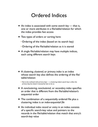
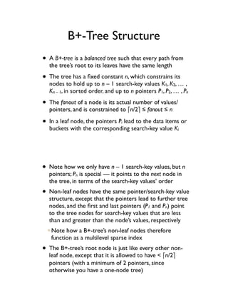
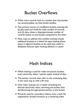
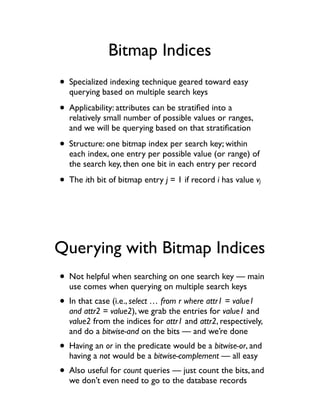
• Alternative to sequential file organization and indices
• A bucket is a unit of storage for one or more records
• If K is the set of all search-key values, and B is the set
of all bucket addresses, we define a hash function as a
function h that maps K to B
• To search for records with search-key value K , wei
calculate h(Ki) and access the bucket at that address
• Can be used for storing data (hash file organization) or
for building indices (hash index organization)
Choosing a Hash Function
• Properties of a good hash function:
Uniform distribution — the same number of search-key
values maps to all buckets for all possible values
Random distribution — on average, at any given time,
each bucket will have the same number of search-key
values, regardless of the current set of values
• Typical hash functions do some computation on the
binary representation of a search key, such as:
31n – 1s[0] + 31n – 2s[1] + !!! + s[n – 1]

11. Bucket Overflows
• When more records hash to a bucket than that bucket
can accommodate, we have bucket overflow
• Two primary causes: (1) insufficient buckets, meaning the
bucket total can’t hold the total number of records,
and (2) skew, where a disproportionate number of
records hashes to one bucket compared to the other
• Many ways to address this: overflow chaining creates
additional buckets in a linked list; open hashing allows
space in adjacent buckets to be used (not useful in
databases because open hashing deletion is a pain)
Hash Indices
• When hashing is used for index structures, buckets
store search-key values + pointer tuples instead of data
• The pointer records then refer to the underlying data,
in the same way as with a B+-tree
• Hash index lookups are a matter of hashing the
desired search-key value, retrieving the bucket, then
dereferencing the appropriate pointer in the bucket
• Primarily used for secondary indices, since a hash file
organization already functions as a clustering index

12. Dynamic Hashing
• Significant issue with static hashing is that the chosen
hash function locks in the maximum number of
buckets a priori — problematic because most real-
world databases grow over time
When the database becomes sufficiently large, we resort to overflow buckets, degrading
performance (i.e., increased I/O to access the overflow chain)
If we hash to a huge number of buckets, there may be a lot of wasted space initially — and
if the database keeps growing, we’ll hit the maximum anyway
• With dynamic hashing, we periodically choose a new
hash function to accommodate changes to the size of
the database
Extendable Hashing
• Extendable hashing chooses a hash function that
generates values over a very large range — the set of
b-bit binary integers, typically b = 32
• The trick to extendable hashing is that we don’t use
the entire range of the hash function right away (that
would be ~4 billion if b = 32!) — instead, we choose a
smaller number of bits, i, and use that initially
• Further, each bucket is associated with a prefix i ! i, j
which allows that bucket to be shared by multiple hash
entries if ij bits can distinguish records in that range

13. Extended Hashing Queries
and Updates
• Queries are straightforward — for search-key value
Kl", the high-order i bits of h(K1) determine the bucket j
• To perform an insertion, write to bucket j if it has
room (recall that j has high-order i bits of h(Kl) only)
If no room, split the bucket and either re-point the hash entry if i > ij or increase i if i = ij
The one case where splitting won’t help is when you simply have more records with Kl
than will fit in a bucket — when this happens, use overflow buckets just as in static hashing
• Deletion goes the other way: if a bucket is empty after
deleting a record, then either decrease the prefix ij or
decrease the overall number of bits i
Static vs. Dynamic Hashing
• Dynamic hashing does not degrade as the database
grows and it has smaller space overhead, at the cost of
increased indirection and implementation complexity
• However, these costs are generally offset by the
degradation experienced when using static hashing, and
so they are considered worthwhile
• Extendable hashing is only one form of dynamic
hashing; there are other techniques in the literature,
such a linear hashing, that improves upon extendable
hashing at the cost of more overflow buckets

14. Ordered Indexing vs. Hashing
• No single answer (sigh); factors include:
The cost of periodic reorganization
Relative frequency of insertion and deletion
Average access time vs. worst-case access time (i.e.,
average access time may be OK but worst-case is
downright nasty)
Types (and frequencies) of queries (see below)
• Most databases implement both B+-trees and hashing,
leaving the final choice to the database designer
• Query types behave very differently under indexing vs.
hashing techniques
For queries where we search based on equality to a
single value (i.e., select … from r where attr = value),
hashing wins because h(value) takes us right to the
bucket that holds the records
For queries where we search based on a range (i.e.,
select … from r where attr ! max and attr # min),
ordered indexing wins because you can find records in
sequence from min up to max, but there is no easy
way to do this with hashing
• Rule of thumb: use ordered indexing unless range
queries will be rare, in which case use hashing

15. Bitmap Indices
• Specialized indexing technique geared toward easy
querying based on multiple search keys
• Applicability: attributes can be stratified into a
relatively small number of possible values or ranges,
and we will be querying based on that stratification
• Structure: one bitmap index per search key; within
each index, one entry per possible value (or range) of
the search key, then one bit in each entry per record
• The ith bit of bitmap entry j = 1 if record i has value v j
Querying with Bitmap Indices
• Not helpful when searching on one search key — main
use comes when querying on multiple search keys
• In that case (i.e., select … from r where attr1 = value1
and attr2 = value2), we grab the entries for value1 and
value2 from the indices for attr1 and attr2, respectively,
and do a bitwise-and on the bits — and we’re done
• Having an or in the predicate would be a bitwise-or, and
having a not would be a bitwise-complement — all easy
• Also useful for count queries — just count the bits, and
we don’t even need to go to the database records

16. Bitmap Index Implementation
• Inserts and deletes would modify the number of bits in
the bitmap entries — inserts aren’t so bad since we
just tack on more bits, but deletes are harder
• Instead of compressing the bits, we can store a
separate existence bitmap, with a 0 in the ith bit if the
ith record has been deleted; then, queries would do a
bitwise-and with the existence bitmap as a last step
• To perform the bitwise operations, we take advantage
of native bitwise instructions, and process things one
word at a time — which today is 32 or 64 bits
Combining Bitmaps
and B+-Trees
• When certain values appear very frequently in a
database, the bitmap technique can be used in a B+-
tree to save space
• Recall that a B+-tree leaf node points to the list of
records whose attribute takes on a particular value
• Instead of one-word-per-record (typical way to store
the record list), do one-bit-per-record, the way it is
done with a bitmap index
• For sufficiently frequent values, the bitmap will be
smaller than the list of records

17. Index Definition in SQL
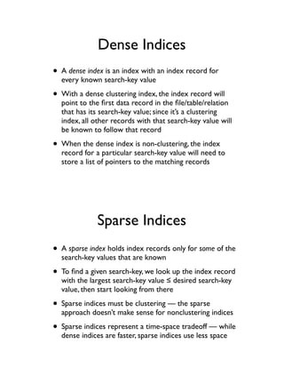
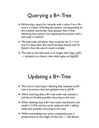
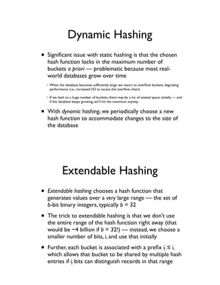
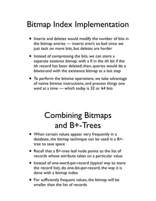
• Because indices only affect efficient implementation
and not correctness, there is no standard SQL way to
control what indices to create and when
• However, because they make such a huge difference in
database performance, an informal create index
command convention does exist:
create [unique] index <name> on <relation> (<attribute_list>)
• Note how an index gets a name; that way, they can be
removed with a drop index <name> command
PostgreSQL Indexing
Specifics
• PostgreSQL creates unique indices for primary keys
• Four types of indices are supported, and you can
specify which to use: B-tree, R-tree, hash, and GiST
(generalized search tree) — default is B-tree, and only B-
tree and GiST can be used for multiple-value indices
• Bitmaps are used for multiple-index queries
• Other interesting index features include: indexing on
expressions instead of just flat values, and partial
indices (i.e., indices that only cover a subset of tuples)